Agriculture is the major sector of Nepalese economy. It provides employment opportunities to around 65 percent of the total population and contributes about 27 percent in the GDP.  Nepalese agriculture has low productivity, depriving farmers of a sustainable livelihood. Especially in the mountains, people who survive by cultivating cereals on mountain slopes, river basins, and small valleys to meet their basic needs, often have low income and suffer from food deficits. Therefore to reduce farm-poverty, the country, through various plans and policies [1-5], identified 'vegetables' as one of the leading sub-sectors to harness the advantages of agro ecological diversity in Nepal. The use of synthetic pesticides in agriculture has increased exponentially after the introduc­tion of high-yielding varieties and hybrids in the late 1940s. At the beginning of the current millennium the world pesticide use exceeded 2.5 million tons and the world pesticide expendi­tures were around $ 32.0 billion [6]. 

Integrated pest management (IPM) technology, a package of practices that utilizes natural predators and careful timing of right doses, is one of the most important measures to cut the use of pesticides. It is not surprising evidence that the application of pesticides during the periods has increased substantially along with incredible amount of subsidies [7]. According to Norton and Mullen [8], IPM is an approach which uses increased information to make pest control decisions, and also uses multiple tactics to manage pest populations in a way that is both economically efficient and ecologically sound. IPM practices natural, environmentally friendly approaches that increase agricultural productivity. Examples of IPM practices are adoption of pest-resistant varieties of crops; biological and physical control methods; environmental modification; bio-pesticides; and when absolutely necessary, non-residual, environmentally-friendly and low mammalian toxic chemical pesticides [9]. The IPM CRSP, began in September 1993 with the objective of developing and implementing IPM practices that can help increase the standard of living and improve the environment in various countries around the world. The objectives areachieved through IPM research, education for behavioral changes, policy and institutional reforms, and the development of sustainable, resource-based local enterprises [10]. The IPM CRSP began its program in Nepal in 2004. The main aim of the study is to compare the farm and household income before and after the adoption of IPM practice. This understanding can help in comparing the income of farm and household and help sustain vegetable production through IPM in Nepal.

Selection of the Study Area

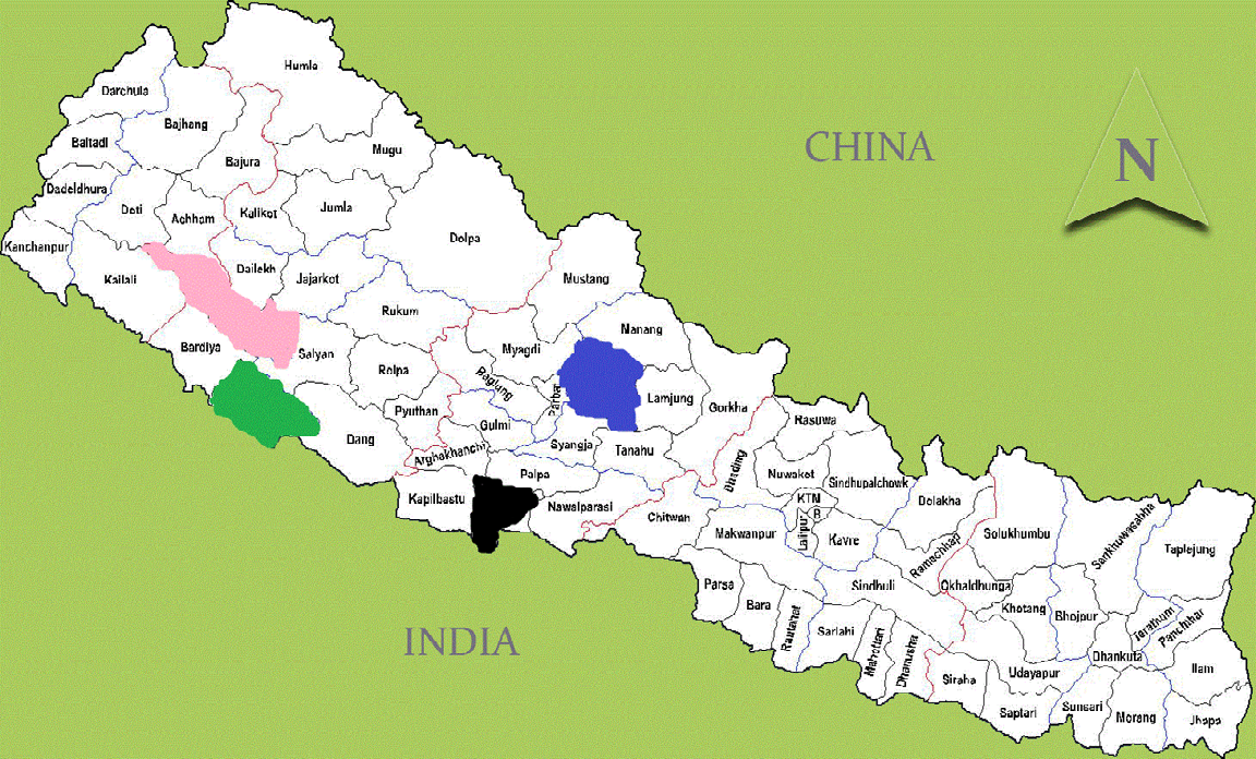
The study was conducted in the mid-western region of Nepal. The study focuses to compare the farm and household income before and after the adoption of IPM technology in, so that, two districts namely Banke and Surkhet were purposively selected (Figure 1).

Figure 1: Map of Nepal Showing Study District

Map of Study Area

The study was conducted in the mid-western development region of Nepal in Banke and Surkhet district. Six Village Development Committees (VDCs) were collected from each district i.e. Banke district:

• Bageshwori

• Kamdi 

• Naubasta

• Sitapur

• Bankatawa 

Basudevpur and in Surkhet Districts:

• Chhinchu

• Dahachaur

• Dashrathpur

• Mehlkuna

• Sahare 

• Malarani

Altogether 500 households were taken, as the sample comprising 42 farmers from   each   VDCs   were   selected randomly which include farmers and marginalized people. Various sources and techniques were used for collection of necessary information. In this study, both primary and secondary data were collected and analyzed. Secondary information were collected from the various published materials like journals, research articles, proceedings of various NGOs and INGOs, reports of District Agriculture Development Office (DADO), District Development Committee (DDC), National Agriculture Research Council (NARC), Central Bureau of Statistics (CBS), Village Development Committee (VDC), Community Development Organizations (CDO), Stattistical year book of Nepal. The local political leaders, working agencies were also the sources of primary information. An interview questionnaire was prepared to collect primary information from farmers.

Lorenz Curve

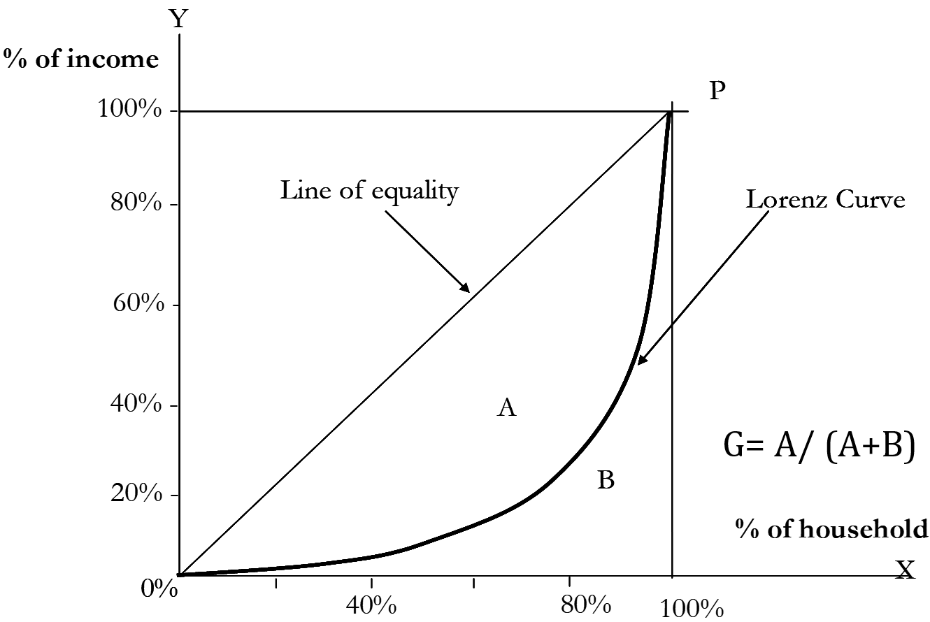
Lorenz curve shows the relationship between the cumulative percentage of aggregate income and the cumulative percentage of the population receiving that income. It indicates the degree of variability of a frequency distribution in a graphical manner. If every member of the population receives the same income, the Lorenz curve will coincide with the line of equal distribution. It means 25 percent of the population receives 25 percent of the aggregate income, 50 percent of the population receives 50 percent of aggregate income and so on [11] (Figure 2).

Figure 2: The Lorenz Curve

To display the disparity in income distribution, Lorenz curve was used. In the figure 1, the curve below the line of inequality indicates the existence of inequity. The more unequal the income distribution, the further below the diagonal (i.e. equalitarian line) will lay the Lorenz Curve.

Gini Coefficient

Gini coefficient was invented by Corrado Gini in 1913 and it is being used with increasing frequency as a measure of relative distributional inequality. The ratio is approximated from the Lorenz curve and represents the portion of area under the egalitarian line that lies between Lorenz curve and egalitarian. It can be clearly defined from the Figure as: 

• G:    A/ (A+B) 
• Mathematically it can be expressed as 
• G:   1/100(∑X_iY_i+1 – ∑X_i+1Y_i) %

Where

• G:    Gini coefficient
• X:     Cumulative percentage of frequency
• Y:     Cumulative percentage of income

The range of Gini coefficient varies from 0 to 1; where 0 indicates perfect equality and 1 indicates perfect inequality.

Fresh Vegetable Crops: District Wise Area, Production and Yield

According to statistical information on Nepalese Agriculture 2075/76, in Surkhet district production of tomato 18.71 mt/ha was high followed by cauliflower 17.25 mt/ha, cabbage     16.46 mt/ha,     cucumber    16.25 mt/ha, brinjal 16.25 mt/ha and bittergourd 15.24 mt/ha. Similarly, in Banke district production of tomato 18.68 mt/ha was high followed by cabbage 17.15 mt/ha, cucumber 16.04 mt/ha, cauliflower 14.94 mt/ha, bittergourd 11.08 mt/ha and brinjal 10.38 mt/ha. The detail of area and production vegetable crops in the study area districts is given in Table 1.

Table 1: District Wise Area, Production and Yield of Fresh Vegetable Crops

Source: Statistical Information on Nepalese Agriculture (2075/76)

Educational Status of the Study Population

Education is one of the important human capitals, which is the main factor of socio-cultural and economic change in a society seven categories, illiterate (who cannot read and write) vocational training (capable of read and write without school), primary (formal education up to five class), secondary (formal education up to ten class), higher secondary (formal education up to twelve class), university undergraduate (formal education up to bachelors level) and university postgraduate (formal education more than bachelors level) were devised in order to assess the educational status of the family members of the sampled households. The survey revealed that large proportion of the members of the sampled households 27.74% have attained secondary level education and lower proportion of the population have attained University post graduate education 1.89%. The illiterate population was higher 18.16% in the Banke district as compared to the Surkhet district 17.06. Lower illiterate population in the Surkhet district may be due to the geographical remoteness. The educational attainment of the members of sampled households was represented in Table 2.

Table 2: Educational Status of the Study Population in the Study Area (2017)

*figures in parentheses indicate percentage

Ethnicity of the Respondent

Majority of the respondents were Janajati/Indigenous followed by Dalit in the study area. In total, 48.6 percentage of   the    respondent    were   Brahmin/Chhetri followed by Janajati/Indigenous 41.6%, Dalit 9.8%. In the Banke district majority of the respondents were Brahmin/Chhetri 50.80% and in Surkhet district majority of the respondents were also Brahmin/Chhetri 46.4%. The distribution of the respondents in the study area was presented in Table 3.

Table 3: Ethnicity of the Respondent in the Study Area (2017)

*Figure in parenthesis indicate the percentage

Distribution of the Economically Active Population in the Study Area

Age of the family members were categorized in to three classes, less than 15 years, economically active age (15-59 year) and more than 59 year. Majority of the population 68.40% was of economically active age. The percentage of economically active population was higher 69.42% in Surkhet district than Banke district 67.49%. Similarly, the percentage of economically active population was higher 57% in Banke district than Surkhet district 53%. The distribution of the economically active population in the study area was presented in Table 4.

Table 4. Economically Active Population in the Study Area 

*Figure in parenthesis indicate the percentage

Cultivation of vegetables

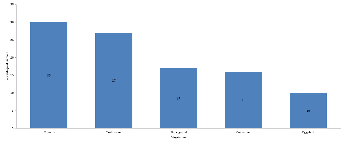
In the study area it has been found that 30% of the household has cultivated tomato followed by cauliflower/cabbage 27%, bitter gourd 17%, cucumber 16% and eggplant 10% respectively. The study revealed that tomato is the major vegetable crops in the study area Figure 3.

Figure 3: Cultivation of Vegetables

Calculation of Benefit Cost (B:C) Ratio Using IPM Technology in The Study Area

In the study area it has been revealed that the benefit cost ratio of cucumber 2.14 was higher followed by tomato 2.11, eggplant 1.92, cauliflower 1.92 and bitter gourd 1.9 in Surkhet district by adopting IPM technology. Similarly, the benefit cost ratio of cucumber 2.01 was higher followed by cauliflower 1.97, tomato 1.93, bitter gourd 1.75 and eggplant 1.29 in Banke district. Hence, cucumber is the most profitable vegetable crops in the study area using IPM technology Table 5.

Table 5: Benefit Cost Ratio of Different Vegetable Crops

Income Distribution of Farm and Households Before and After Adoption of IPM Practice

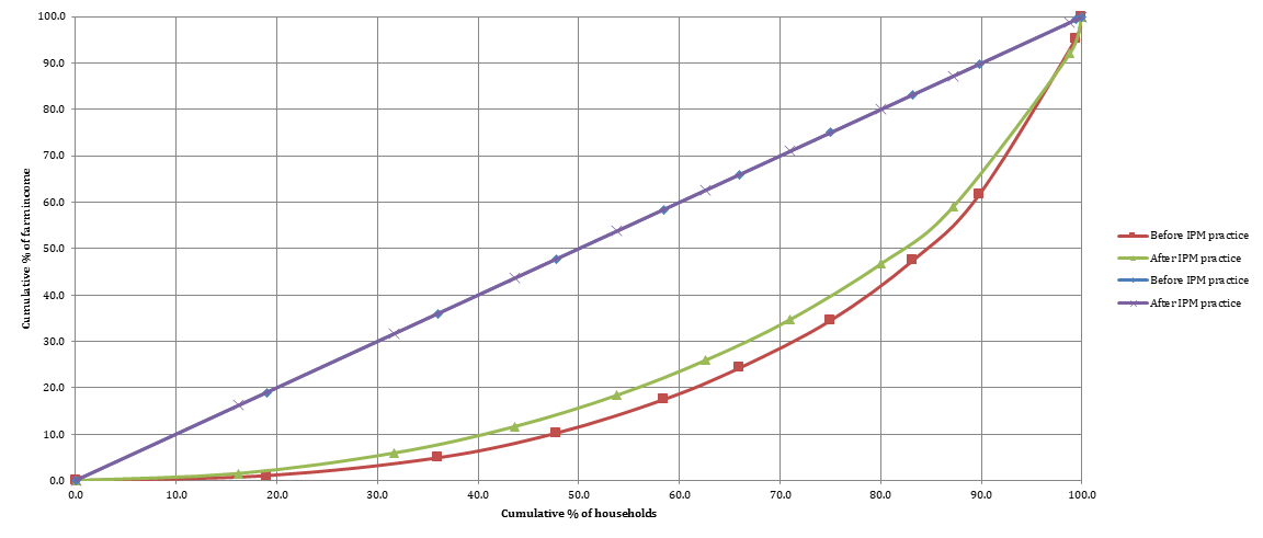
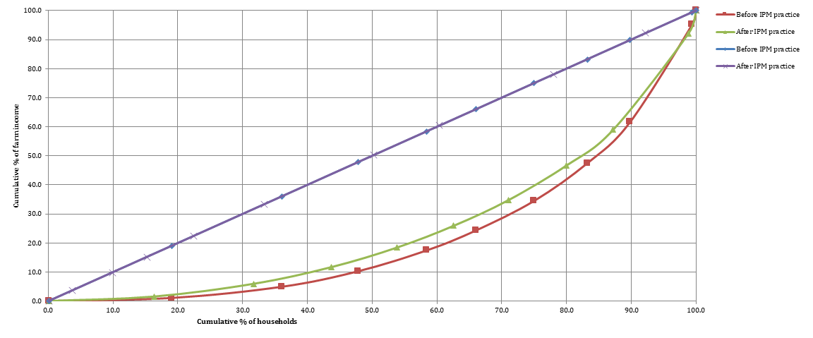
Distribution of Farm Incomes Before and After Adoption of IPM Practice: The figure presented below is the farm income distribution of sample households before and after adoption of IPM practice. Lorenz curve (Figure 4) presents the disparity of farm income distribution before and after adoption of IPM practice. The farm income of sample households before IPM practice ranged from Rs. 2,150 to Rs. 466,000. The poorest 19 percent of the households had access to only 1.1 percent of the cumulative farm income and the richest 0.6 percent had earned 4.8 percent of the cumulative farm income. Likewise, lower 58.4 percent of the households earned only 17.4 percent whereas upper 41.6 percent earned 82.6 percent of the cumulative farm income before adoption of IPM practice. After the adoption of IPM practice, the farm income ranged from Rs. 5,500 to Rs. 499,000. The poorest 16.2 percent of the households had access to only 1.5 percent of the cumulative farm income and the richest 1.2 percent had earned 8 percent of the cumulative farm income. Likewise, lower 53.8 percent of the households earned only 18.4 percent whereas upper 46.2 percent earned 81.6 percent of the cumulative farm income after IPM practice adoption.

Figure 4: Lorenz Curve for Distribution of Farm Incomes of Households

Distribution of Household Incomes Before and After Adoption of IPM Practice

The figure presented below shows the household income distribution of sample households before and after IPM practice adoption. Lorenz curve (Figure 5) presents the disparity of household income distribution before and after IPM practice adoption. The household income of sample households before adoption of IPM practice ranged from Rs. 23,000 to Rs. 647,000. The poorest 5 percent of the households had access to only 0.4 percent of the cumulative household income and the richest 7.4 percent had earned 21.9 percent of the cumulative household income. Likewise, lower 53.8 percent of the households earned only 27.4 percent whereas upper 46.2 percent earned 72.6 percent of the cumulative household income before IPM practice adoption. After the adoption of IPM practice, the household income ranged from Rs. 25,000 to Rs. 696,000. The poorest 3.6 percent of the households had access to only 0.2 percent of the cumulative household income and the richest 7.8 percent had earned 17.6 percent of the cumulative household income. Likewise, lower 50 percent of the households earned only 27.7 percent whereas upper 50 percent earned 72.3 percent of the cumulative household income after IPM practice adoption.

Figure 5: Lorenz Curve for Distribution of Household Incomes of Households

Gini Coefficient

Gini coefficients explain the equality and inequality in farm and household income distributions of the households in the study area. It was revealed that the disparity of farm and household income prevailed both before and after IPM practice adoptions in the farms of the households Table 6. The Gini coefficients were higher for farm income 0.55 and household income 0.37 before adoption of IPM practice compared to those for farm income 0.49 and household income 0.31 after adoption of IPM practice. Since the Lorenz curves (Figures 4 and 5) for both farm and household incomes after IPM practice lie close to the line of equality compared to those before IPM practice, disparity of income was reduced after the provision of IPM practice. Disparity of farm income was reduced significantly compared to household income.

Table 6: Gini Coefficients for Farm and Household Income Disparities

Summary

Integrated pest management (IPM) technology, a package of practices that utilizes natural predators and careful timing of right doses, is one of the most important measures to cut the use of pesticides. It is not surprising evidence that the application of pesticides during the periods has increased substantially along with incredible amount of subsidies. A study on comparison on farm income and household income before and after adoption of IPM technology was conducted in the Banke and Surkhet districts of Nepal. For assessing the comparison, farmers were asked a series of questions during the survey to determine the income before and after IPM adoption. For the comparison Lorenz curve and Gini coefficient were used. This study revealed that that large proportion of the members of the sampled households (27.74%) has attained secondary level. Majority of the respondents were Janajati/Indigenous followed by Dalit in the study area 68.40% population were of economically active age. Similarly, 30% of the household has cultivated tomato followed by cauliflower (27%), bitter gourd (17%), cucumber (16%) and eggplant (10%). Cucumber is found to be the most profitable vegetable crops in the study area using IPM technology. The farm income of sample households before IPM practice ranged from Rs. 2,150 to Rs. 466,000 and after the adoption of IPM practice, the farm income ranged from Rs. 5,500 to Rs. 499,000. Similarly, the household income of sample households before adoption of IPM practice ranged from Rs. 23,000 to Rs. 647,000 and after the adoption of IPM practice, the household income ranged from Rs. 25,000 to Rs. 696,000. The Gini coefficients were higher for farm income (0.55) and household income (0.37) before adoption of IPM practice compared to those for farm income (0.49) and household income (0.31) after adoption of IPM practice. Since the Lorenz curves for both farm and household incomes after IPM practice lie close to the line of equality compared to those before IPM practice, disparity of income was reduced after the provision of IPM practice. Disparity of farm income was reduced significantly compared to household income. Thus, identified comparison of farm and household income before and after adoption of IPM practice could be a source for Agriculture Knowledge Centers, policy makers, researchers and other extension agents to disseminate the IPM technology.

1. National Planning Commission (NPC). Nepal agriculture perspective plan. National Planning Commission and Asian Development Bank, 1995.

2. National Planning Commission (NPC). The ninth plan. National Planning Commission, 1998.

3. National Planning Commission (NPC). The tenth plan. National Planning Commission, 2003.

4. National Planning Commission (NPC). Three years interim plan. National Planning Commission, 2007.

5. Ministry of Agriculture and Cooperative (MOAC). National agricultural policy. MOAC, 2004.

6. Environmental Protection Agency (EPA). What is IPM. Environmental Protection Agency, 2002.

7. Irham, and J. Mariyono. “The impact of integrated pest management on pesticide demand for soybean farming in Yogyakarta, Indonesia.” Proceedings of the International Workshop on Environmental Risk Assessment of Pesticides and Integrated Pesticide Management in Developing Countries, edited by A. Herrmann and S. Schumann, Landschaftsökologie und Umweltforschung, vol. 38, 2002, pp. 62–72.

8. Norton, G.W. and J. Mullen. “Economic evaluation of integrated pest management programs: A literature review.” MS thesis, Virginia Polytechnic Institute and State University, 1994.

9. IPM CRSP. What do we do. IPM CRSP, 2008.

10. IPM CRSP. IPM CRSP IPM goals and objectives. IPM CRSP, 2008.

11. Riston, C. Agricultural economics: Principles and policy. Granada Publishing, 1977, pp. 30–38