Numerical Methods exist to calculate single Integrals, which are specified in their integration periods.

• Trapezoidal Rule

• Midpoint Rule

• Simpson’s Rule

• Simpson’s Rule 8/3 called Newton-Coates formats

In this research we will address the Simpson 3/8 method of finding rough values for mono complementarities.

The same continuous supplements using the triangular acceleration methods of the meme and we will compare these methods with each other to select the best ones in terms of accuracy and speed at which the values of these methods approach the real (analytical) values of those complementarities.

Let's assume integration J as follows:

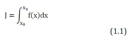
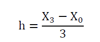
where, f (x) continuous supplement is located above the x axis in the [x_0, x_3] period and what is required is to calculate the J value approximately. Generally speaking, Newton-Coates integration formats (1) can be written as follows [1]: 

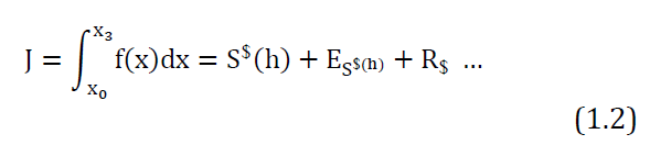
where, S^$ $ represents the Lagrangian-Approximation of the Integrative Value of Jas, E_s$(h)  is the series of correction limits that can be added to the values of R_$ is the remainder that the value of S* (h) symbol to the base of the Semsonzone.

when:

The general formulation of E_S^$ (h) is as follows [2].

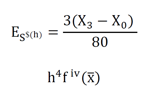
So when Al-Karamy [3] full integration is a continuous function and its derivatives are present at each integration period point [x_0, x_3], we can write the error form.

where, An A₁, A₂, A₃ Constants whose values depend not on h but on the values of the derivatives of the function at the end of two periods.

Integration and J real value (set) for integration.

Accelerating the Triangular Functions of Simpson Rule 8/3

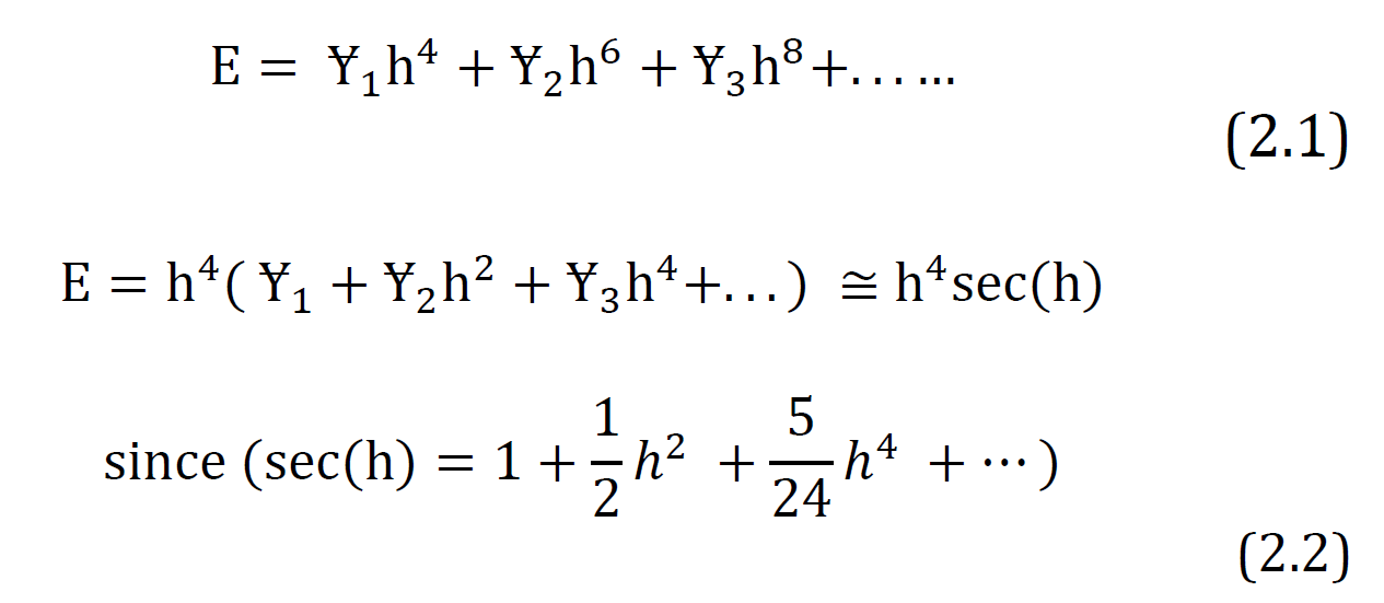
We will now address accelerative methods that we call trigonometric accelerators [4].

We note that:

Assuming that S to S^$ (h) is the approximate value of integration, the Simpson base is 3/8:

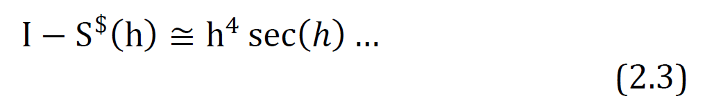
If we impose two values to J numerically at Simpson's base 3/8. S^$ (h₁) when h = h₁ and S^$ (h₂):

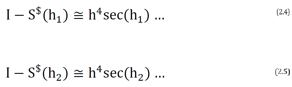
Of the formulas (2.4) and (2.5) we get:

We call the formula (2.6) the first trigonometric cutter law and we symbolized it as a symbol (AE^S$ _sec).

Similarly, the second accelerated triangular law can be written if the E error can be written in the above as follows.

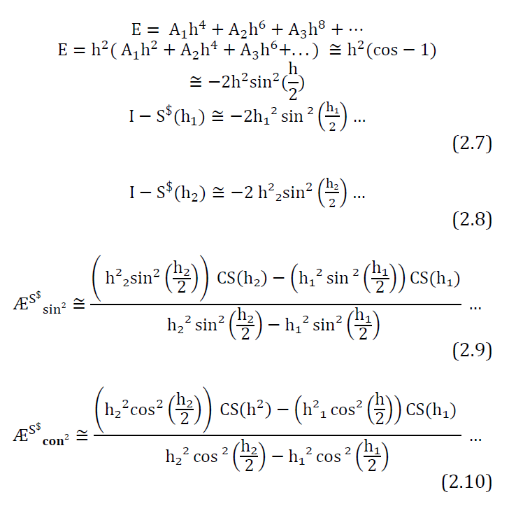
We call version No. 2.10 a law for the quadratic, accelerated pocket.

Examples

Based on the foregoing, we will address some complementarities that continue in the integration period and use triangular acceleration methods to improve the outcomes for complementarities below.

Thus, the tables of the six accelerated methods are compared once with the Simpson base three eighth and the other with each other and the preference for the accelerated method is calculated based on n values n = 3,6,9…, The results we adopted in the Matlab programmer ^12-10=Eps.

Findings

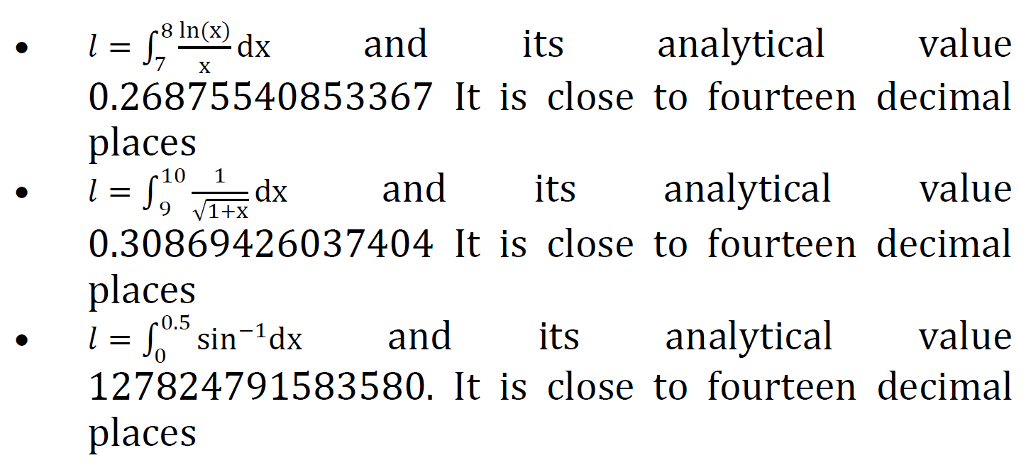
The Integration Integrator

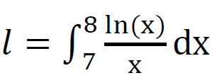
Continuous in the integration period 7.8 The correction limits formula of Simpson Rule 3/8 as in version 1.3 (Table 1).

Table 1: Integration Account Numerically using the Simpson Base Three Eight with Accelerated Triangular Functions

N	Values of simpson’s 3/8 rule
3	0.268755
6	0.268755	0.268755	0.268755	0.268755
9	0.268755	0.268755	0.268755	0.268755
12	0.268755	0.268755	0.268755	0.268755
15	0.268755	0.268755	0.268755	0.268755

This example is a solution in the message (innovative acceleration methods for second-class mascots to improve the results of numerically integrative values) that gave accuracy of the Simpson method without acceleration to nine decimal places while using accelerations we obtained valid values to twelve decimal places [5,6]. While our method got a valid value by accelerating theto thirteen decimal places when n = 15 as well as for other accelerations while the Simpson value was three eight without acceleration was correct to ten decimal places when n = 15.

The Integration Integrator continuous in the integration period and the correction limits formula of the Simpson3/8 rule as in the version No. (1.3) (Table 2).

Table 2: Integration Account Numerically using the Simpson Base Three Eight with Accelerated Trigonometric Functions

N	Values of simpson’s 3/8 rule
3	0.308694
6	0.308694	0.308694	0.308694	0.308694
9	0.308694	0.308694	0.308694	0.308694
12	0.308694	0.308694	0.308694	0.308694
15	0.308694			0.308694

This example is a solution in the message (innovative acceleration methods for second-class mascots to improve the results of numerically integrative values) that gave accuracy of the Simpson method without acceleration to ten decimal places and using accelerations we obtained two decimal places [5,6]. While our method got valuable by accelerating to thirteen decimal places when n = 12 as well as for other accelerators while the Simpson value is three eight without acceleration was correct to nine decimal places when n = 15 except acceleration:

We got thirteen decimal places when n = 15.

The Integration Integrator continuous in the integration period [0.0.5] and the correction limits formula of the Simpson Rule 3/8 as in the version No. (1) (Table 3).

Table 3: Integration Account Numerically using the Simpson Base Three Eight with accelerated Trigonometric Functions

N	Values of simpson’s 3/8 rule
3	0.127841
6	0.127826	0.127825	0.127825	0.127825
9	0.127825	0.127825	0.127825	0.127825
12	0.127825	0.127825	0.127825	0.127825
15	0.127825	0.127825	0.127825	0.127825
18	0.127825	0.127825	0.127825	0.127825
21	0.127825	0.127825	0.127825	0.127825
24	0.127825	0.127825	0.127825	0.127825
27	0.127825	0.127825	0.127825	0.127825
30	0.127825	0.127825	0.127825	0.127825
33	0.127825	0.127825	0.127825	0.127825
36	0.127825	0.127825	0.127825	0.127825

This example is a solution in the message (innovative acceleration methods for second-class meme to improve the results of numerically integrative values) that gave accuracy by accelerating A^SCOS(h) And the other accelerators to eleven decimal places while the Simpsons without acceleration were correct to eight decimal places [5,6], while our method gave precision by accelerating . To eleven decimal places when n = 3 and so for the other accelerators while in Simpson's way three eight without haste we got eight decimal places when n = 36.

From the tables above, we conclude that these accelerative methods operate with the same efficiency and give high accuracy in results and relatively few partial periods.

1. Fox, Leslie and Linda Hayes. “On the Definite Integration of Singular Integrands.” SIAM Review, vol. 12, no. 3, 1970, pp. 449-457.

2. Sastry, S.S. Introductory Methods of Numerical Analysis. PHI Learning Pvt. Ltd., 2012.

3. Al-Karamy, N. “New Acceleration Formule for Improvement Results of the Numerical Integrations.” Journal of Kerbala University, vol. 15, no. 2, 2017.

4. Zwillinger, D. CRC Standard Mathematical Tables and Formulae. Zwillinger, D. Ed. CRC Press, 2002.

5. Chadha, Haider et al. Innovative Acceleration Methods for Second-Class Mascots to Improve Outcomes of Values of Numerically Integrations. Master’s Thesis, University of Koufa, 2020.

6. Asmahan, Abd Yasser and Al-Shammari. Innovative Acceleration Methods for First-Class Masters to Improve Values of Numerically Integrations. Master’s Thesis, Koufa University, 2019.