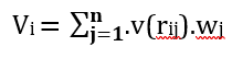
Basic Revive Mathematical Integration: The following is a general formulation of the numerical integration problem: an assortment of data points  

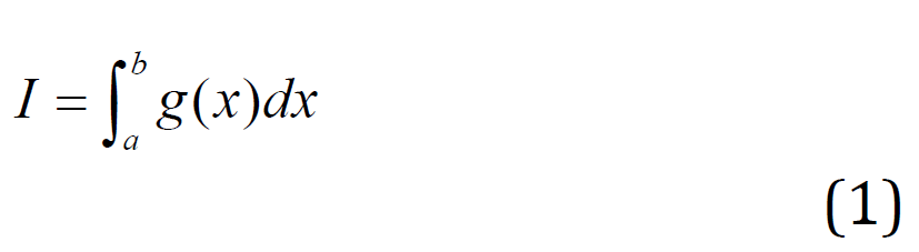
It is necessary to calculate the definite integral's value as follows:

One replaces the other, just like in the case of numerical differentiation. f(x) by a polynomial interpolator. Æ(x) and succeeds on integration  a rough estimate obtained depending upon the type of the interpolation Depending on the interpolation formula utilized, formulas can be produced. Using Newton's forward difference formula, a general formula for numerical integration will be derived in this section [21]. 

Let's divide the range [a, b] into n equal subranges so that 

The integral follows:

Approximating f(x) Newton's forward difference formula yields the following:

Since, x = x₀ + uh, dx = hdu and as a result, the above integral is:

which focuses on simplifying:

Using this basic formula By entering n = 1, 2, 3,..., ets, we can get several integration equations. Some of these formulas, like the trapezoidal and Simpson's 1/3-rules, which are determined to have sufficient precision to be applied in real-world situations, can be derived here [19].

With n = 3, we can see that any differences higher than the third will be zero in Eq. (1.5) and the integral will then be [22]:

Similarly:

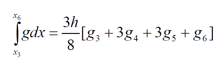
And so on. Summing up all these integral formulas, we obtain:

This rule, often known as Simpson's (3/8) rule, is not quite as precise.

The primary term in this formula's inaccuracy is:

Matlab Algorithm

Working algorithm calcation of Dental ceries Area.

Determining and Calculating the Area of Tooth Decay

The purpose of this application is to build a program that deals with medical images whose area is difficult to calculate [3]. After determining the caries area, taking a picture of the caries area, determining it with points on the edges of the image with the mouse and then calculating the decay area for the irregular shape according to Figure 1,

And Figure 2 by applying the Simpson method 1/3 or the proposed method for calculating the area as shown in the following examples [15].

Determine the Thrombus Area in the Artery

Determining and calculating the arterial thrombus area and the area of pneumonia.

The purpose of this application is to build a program that deals with medical images as well. The area of which is difficult to calculate using the usual methods [3] after taking a picture of the blood clot in the artery by using colored rays through which it is possible to identify or locate the clot. Also, a picture of the pneumonia of the infected person can be taken. Determining the area of inflammation through which the poor pathological condition can be known, after locating the edges of the image with points of irregular shape and then the area can be calculated by applying the Simpson 3/8 method or the proposed method for calculating the area as shown in the following examples [13].

Matlab Coud

The area of irregular shapes in images can be calculated using Simpson's octet equation. It is worth noting that Simpson's eight equation is usually used to divide curved areas into small parts and calculate the area of each part and it is one of the most common methods for calculating areas in mathematics and engineering. To apply Simpson's eight equations to irregular images, a mathematical computing program such as Matlab can be used:

clc ;

clear ; 

close all ;

clf

hold on

z=imread('p5.jpg');

image(z);

grid

echo on

 x = []; y = []; n = 0; % Loop, picking up the points. 

but = 1; 

echo off;

while but == 1 

    [xi,yi,but] = ginput(1);

    if length(but)==0

        if n<2 

            but=1;

            disp('Pick at least two points please.')

        else

            but=2;

        end

    elseif but~=1

        if n<11

            but=1;

            disp('Pick at least two points please.')

        end

plot(xi,yi,'g*')

grid

n = n + 1;

text(xi,yi,[' ' int2str(n)],'Erase','back');

x = [x; xi];

y = [y; yi];

end

end

echo on;

disp('End of data entry')

% pause

 clc

n=n+1;

x = [x; x(1)];

y = [y; y(1)];

% Interpolate the points with two splines

t = 1:n;

ts = 1:1/10:n;

xs = pchip(t,x,ts);

ys = pchip(t,y,ts);

% pause

% xs = [xs xs(1)];

% ys = [ys ys(1)];

% Plot the interpolated curve. 

plot(xs,ys,'r-');

NoOfLevels=1;

inv =0;

cornars=[];

for i=2:length(xs)

    if xs(i)<xs(i-1) && inv==0

       NoOfLevels = NoOfLevels+1; 

       inv=1;

       cornars =[cornars i];

    elseif xs(i)>xs(i-1)&& inv==1

        NoOfLevels = NoOfLevels+1;

        inv=0;

        cornars =[cornars i];

    end

end

area=0;

for j=1:NoOfLevels

    if j==1

        a=xs(1);

        b=xs(cornars(1));

        fun= ys(1:cornars(1));

    elseif j==NoOfLevels

        a=xs(cornars(j-1)+1);

        b=xs(end);

        fun= ys(cornars(j-1)+1:end);

    else

        a=xs(cornars(j-1)+1);

        b=xs(cornars(j));

        fun= ys(cornars(j-1)+1:cornars(j));

    end

       IS_EVEN = ~mod(j,2);

    if IS_EVEN ==0

        area = area + simpsons(fun,a,b,[]);

    else

        area = area - simpsons(flip(fun),b,a,[]);

    end

   end

% area=abs(trapz(xs,ys));

echo off

hold off

disp('End')

The research aims to develop a program that deals with medical images and calculates the area of those images in a simple way using the calculator after determining [9] the dimensions of those images on an axis x and an axis y, then calculating the area of the irregular shape after relying on the Simpson 3/8 method. Which is considered one of the methods of numerical integration with high accuracy in calculating the area of the irregular shape and an error rate less than the method of the trapezoid, which is considered one of the primitive methods in calculating the values of numerical integrations, as well as any other method of numerical integration. Methods can be added to the program that calculates the area by specifying points with the mouse for irregular shapes and dimensions. The image whose area is to be calculated.

1. Alusian, A. et al. Introduction to Numerical Analysis. Bagudad Is the Home of Ibn Al-Atheer for Printing and Publishing, 1989, pp. 31–40, 2–343.

2. Brezinski, C. “Convergence Acceleration during the 20th Century.” Numerical Analysis: Historical Developments in the 20th Century, 2001, p. 113.

3. Deplazes. “Apical Transportation, NiTi Instruments.” Journal of Endodontics, vol. 27, no. 3, March 2001.

4. Davis, P.J. and P. Rabinowitz. Numerical Integration: Waltham–Toronto–London. Blaisdell Publishing, 1967.

5. Balogurusam, E. Numerical Methods. Tata McGraw-Hill, 1999, pp. 386–407, 2–608.

6. Fox, L. “Romberg Integration for a Class of Singular Integrands.” The Computer Journal, vol. 10, no. 1, 1967, pp. 87–93.

7. Hamming, R.W. and R.S. Pinkham. “A Class of Integration Formulas.” Journal of the ACM, vol. 13, no. 3, 1966, pp. 430–438.

8. Ferziger, J.H. Numerical Methods for Engineering Application. 1981.

9. Kwak, T.A. W-Sn Skarn Deposits: And Related Metamorphic Skarns and Granitoids. Elsevier, 2012.

10. Mohammed, A.H. and S.H. Theyab. “Relative and Logarithmic of Al-Tememe Acceleration Methods for Improving the Values of Integrations Numerically of Second Kind.” 2019.

11. Perhiyar, M.A. et al. “Modified Trapezoidal Rule Based Different Averages for Numerical Integration.” 2019.

12. Matlab User’s Guide. Mathsoft, ver. 6.0, 2000.

13. Opie, L.H., Heart Physiology: From Cell to Circulation. Lippincott Williams and Wilkins, 2004.

14. Povicic, J. et al. “Application of Simpson’s and Trapezoidal Formulas for Volume Calculation of Subsurface Structures.” Original Scientific, 2018.

15. Gonzalez, R.C. Digital Image Processing. 1987.

16. Ramachandran, T. et al. “Centroidal Mean Derivative-Based Closed Newton Cotes Quadrature.” International Journal of Science and Research, 2016.

17. Ramachandran, T. et al. “Comparison of Arithmetic Mean, Geometric Mean and Harmonic Mean Derivative-Based Closed Newton Cotes Quadrature.” Progress in Nonlinear Dynamics and Chaos, vol. 4, 2016, pp. 35–43.

18. Romberg, W. “Vereinfachte Numerische Integration.” Norske Vidensk. Selsk. Forh., vol. 28, 1955, pp. 30–36.

19. Chapra, S.C. and R.P. Canale. Numerical Methods for Engineers. 6th Edn., 2010, pp. 600–630.

20. Shanks, J.A. “Romberg Tables for Singular Integrands.” The Computer Journal, vol. 15, no. 4, 1972, pp. 360–361.

21. Sastry, S.S. Introductory Methods of Numerical Analysis. 5th Edn., 2012, pp. 207–254.

22. Sastry, S.S. Introductory Methods of Numerical Analysis. PHI Learning, 2012.

23. Tyler, G.W. “Numerical Integration of Functions of Several Variables.” Canadian Journal of Mathematics, vol. 5, 1953, pp. 393–412.

24. Tomashefski, J.F. et al. Dail and Hammar’s Pulmonary Pathology: Volume I: Nonneoplastic Lung Disease. Springer, 2008.