In the context of intense competition in the manufacturing industry, companies are looking to achieve low-cost production through effective planning and management techniques. However, due to abnormal customer demand, the current production scheduling and inventory management model of a packaging manufacturing company is not effective which results in high inventory costs. 

Related to this problem, there are many studies of demand forecasting and inventory management around the world. In the demand forecasting field, there are some practical application cases such as a model is developed to determine the most appropriate forecasting method based on forecast errors at a manufacturing company in Bangladesh [1]. According to Beutel et al. [2], authors discussed a framework of least squares demand forecasting and inventory decision making. Demand patterns also plays an essential role for companies to identify level of inventory. Based on demand data, an appropriate inventory model is conducted [3]. Besides, safety stock should be considered in inventory planning model to avoid the risk of shortage stock [4]. There are many safety stock calculating formulas. For instance, some safety stock formulas are based on the distribution of the total demand in a lead time and the standard deviation of total demand in a lead time [5,6].

Actually, the problem of demand management and inventory planning is widely discussed, which create a premise for the case study of this article. Originating from the production-inventory model at a packaging manufacturing company, this research was carried out, contributing to the diversity in the field. 

The research intends to achieve four objectives. First, the inventory status of the research object was analyzed and evaluated. Second, customer demand through analysis of historical sales data was managed in the suitable forecasting models. Third, a suitable inventory model to reduce the total cost of inventory was proposed. It ensures that the new model does not increase the company's inventory cost. Last, the evaluation of the solution model is the basis to show that this model could be applied in practice at the studied company.

In the next section, the previous research related to this problem was summarized. Section three focuses on analyzing the case study, collecting and analyzing data to identify problems. The next two sections are to propose a solution model using forecast techniques and economics production quantity model. For the last section, the research results were discussed and some recommendations were introduced for the studies in the future.

Demand patterns also play an essential role for companies to identify level of inventory. Specifically for companies with dynamic one, mismanagement of inventory level could consequently be more tremendous, hence appropriate forecasting technique is imperative for such companies and one of the most effective software to support forecasting is processed with Minitab software [1,7,8]. The authors analyzed eight different forecasting techniques including the Simple Moving Average, Single Exponential Smoothing, Trend Analysis, Winters method and Holt's method with Minitab 17 software. The effectiveness of the above methods is evaluated on the basis of the accuracy of the forecast and the analysis shows that the Winters model is the best based on the errors. Also, with Minitab software, a study on a model to forecast the increase in the number of COVID-19 infections through seven different forecasting methods [8]. In this study, the appropriate forecasting techniques would be used. The forecasting technique procedure has three main steps including analyzing the data characteristics and time series, choosing and implementing appropriate forecast methods, evaluating forecasting errors and verifying forecasting models by residual analysis [9].

Besides, inventory management plays an indispensable role in any manufacturing company. The profound objective of inventory management is no other than enhancing competitive advantage for businesses through cutting down excessive cost and maintaining a desired customer service level. The determination of whether to apply which of inventory policies for a certain warehouse relies on several factor, such as product attribute, demand pattern, warehouse operation, supply contracts and manufacturing capacity [3,10-13]. Related to this problem, a comparison of the effectiveness between the two most common inventory control policies, Continuous Review Policy and Periodic Review Policy, was done under the condition of dynamic demand characteristic within an automotive company in Indonesia [14]. The comparison criteria among the two mentioned policies were the total inventory cost of the company. The result shows that total inventory cost of the Continuous Policy was lower than that of the Periodic Review Policy by 53.89%. A vendor-managed inventory model in the manufacturing industry was developed with a mathematical model to achieve the objective of minimizing total inventory cost of the supply chain and maximize customer service level [15].

In inventory planning model, safety stock, an indicator to determine the minimum amount of stock to satisfy customer service, is also an essential metric to be considered. For the majority of cases, the optimal degree of safety stock is based on forecasts of up-coming demands. There are many safety stock calculating formulas. For instance, some safety stock formulas are based on the distribution of the total demand in a lead time and the standard deviation of total demand in a lead time [2,5,6]. A model that considers both direct and indirect costs related to inventory to calculate safety stock was presented in [4]. Besides, safety stock formulas were defined through safety factor, standard deviation of demand per unit time, total review period and lead time [13].

Most previous related studies showed a similar approach that promoting integrated causal demand forecasting and inventory management. Depending on the practical case studies, there are some differences of factors in solution models. Based on the literature review, an attempt was made to create and implement a review policy for sustaining a better level of finished goods inventory in the local company, the manufacturer of carton packaging.

The methodology is visualized as in flowchart (Figure 1). Our methodology starts with simultaneously analyzing company operations and reviewing the relevant research. Some data are collected in this stage to determine the problem of company operation. Then, fish bone diagram and Pareto chart are applied to define and analyze root causes of this problem. Next, solutions for the problem are proposed based on root causes, including demand management by forecasting techniques and appropriate inventory planning model, to determine whether the solution should be implemented to eliminate the root causes. Finally, the evaluation is carried out to ensure the efficiency of our solution in the last stages. Each process to do the research would be mentioned in relative following sections.

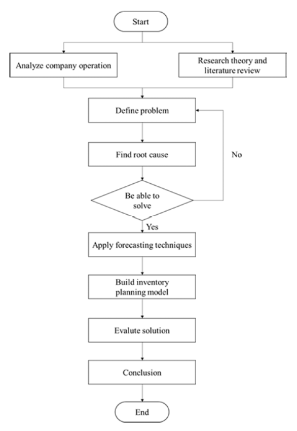
Figure 1: Research Methodology

Problem Description

Overview: The research object is a company specializing in carton manufacturing. This company has more than 20 years of experience within the field and currently employing more than 400 employees. The company is currently facing the problem of high inventory cost, compared to the company’s product’s price. Furthermore, it is notable that the research company’s selling prices are the highest among its rival, which is indeed a circumstance for the company’s competitive advantage in Vietnam market.

It is obvious that besides manufacturing cost (accounted for nearly 30% of selling price), sales cost is the second highest component comprising 23% of the total selling price. Sales cost comprises many components, such as transportation cost, marketing cost, inventory cost and other costs. In which, inventory cost and transportation cost are the two highest components, accounting for 36 and 30% of the total sales cost respectively. However, there are many external factors affecting to transportation cost. On the other hand, inventory cost is an internal factor, which can be improved to lower sales cost and selling price.

Current Inventory Policy Analysis

Currently, the company manages inventory based on experience. The inventory level is set for each product at a certain quantity and weekly reviewed, then issue production orders to keep that level of inventory at all times. However, a fixed inventory level is too high, compared with actual sales. Although the fixed inventory level is easy to manage, it is leading to a large amount of unnecessary inventory, which increases the inventory cost of company. Historical sales and inventory data shows that weekly average waste stocks range from 79 to 84%.

Root Cause Analysis

By surveying experts’ ideas, such as factory manager, production manager, team leaders and planner staffs, the causes affecting the inventory cost are shown in the fishbone diagram as Figure 2.

Figure 2 presents four main causes (environment, technology and machine, method and man) relating to the problem “High inventory cost”. Each cause comprises of different subordinate causes. Theses subordinate causes are evaluated by FMEA (Failure-Mode-Effect Analysis) technique. The Risk Priority Number (RPN) is an important element using in FMEA technique. RPN factor can be easily calculated by multiplying three criteria, namely SEV (Severity), OCC (Occurrence) and DET (Detection). The weighted points are also assessed by experts’ ideas. The accumulation of FMEA analysis is presented visually by a Pareto chart presented in Figure 3.

The result indicates that the top three causes accounting more than 50% of the problem “High inventory cost” are Inappropriate inventory planning method (22.27%), Inappropriate forecast (16.7%) and Demand volatility (10.61%).

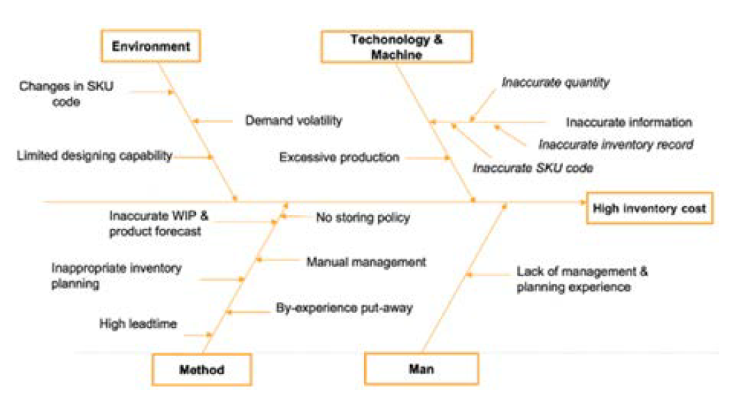
Figure 2: Fish Bone Diagram Analyzing “High Inventory Cost” Problem

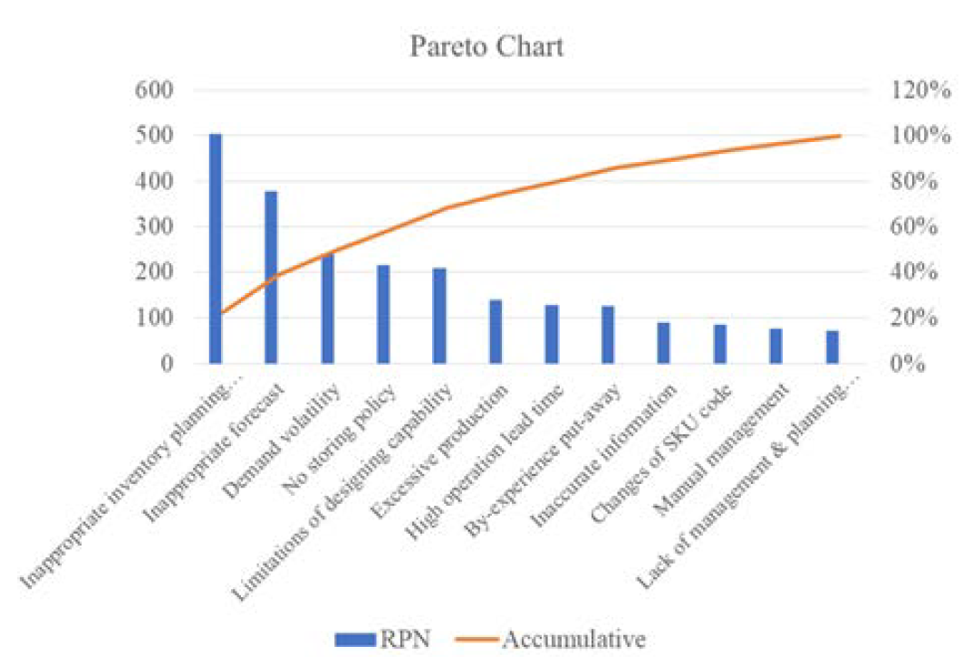
Figure 3: Pareto Chart Summarizing FMEA Result

Proposed Solution

Demand volatility is regarded to be an external factor. Therefore, this study focuses on solving the other two problems: Inappropriate inventory planning method and Inappropriate forecast through forecasting techniques and inventory planning model. The main objectives of the proposed solution is to reduce inventory level, thereby reducing inventory cost, reducing selling price and gaining the company’s competitive advantage.

In our case study, 4 important products of company are focused, which are assessed to have high inventory level. The names of these products are encoded because of company’s private policy, including: Z001, Z002, Z003, Z004.

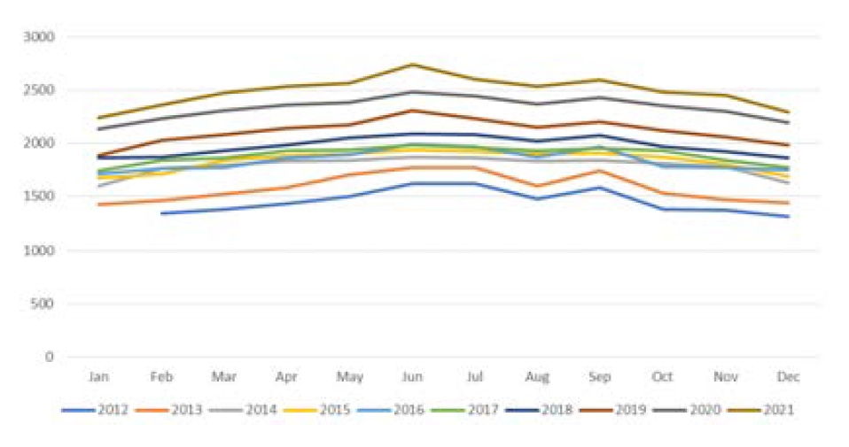
Figure 4: Seasonality Analysis Plot of Z001 Product

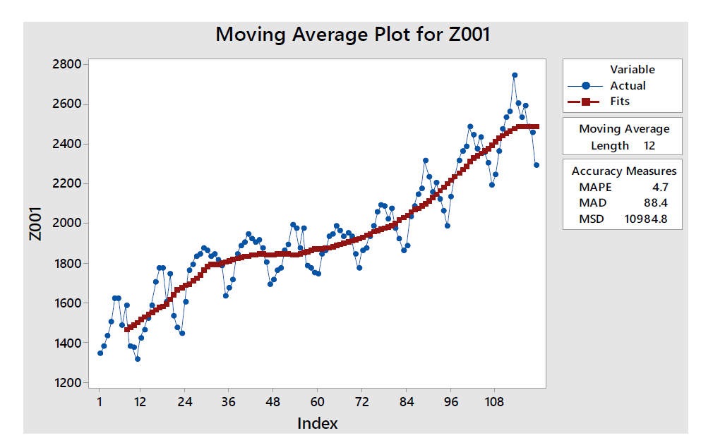
Figure 5: Trend Analysis Using CMA of Z001 Product

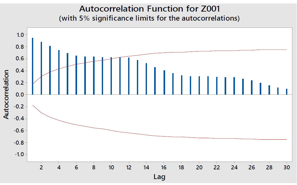
Figure 6: ACF Plot of Z001 Product

Demand Forecast

The forecasting procedure includes these steps: analyzing data characteristics and time series, choosing forecast methods and analyzing residuals (forecasting errors) [9]. In our study, the forecast techniques are carried out through Minitab 17 Software.

Time series plots show that all products demand has uptrend and seasonal pattern. For example, to conduct the trend and seasonality of Z001 product, we summarize data in month per year. The seasonality analysis chart shows that the data has same pattern through years, so the product is seasonal with a cycle of 12 months (Figure 4).

Because the seasonal length is 12 month, to determine the trend of data, we use Centered Moving Average (CMA) method with k = 12 (Figure 5), the plot show that the trend of Z001 product is increasing.

The seasonality and the trend of data will be verified through the autocorrelation plot (ACF) as shown in Figure 6.

According to Hanke and Wichern [9], the autocorrelation coefficients decrease to zero with increasing lag, demonstrating that this data has trend characteristic. Also, considering about 12 lags, the graph has similar shape, so this data is seasonal with a seasonal length of 12 periods.

Because of the trend and seasonality of the data, some forecasting methods suitable for the model are ARIMA method (Box-Jenkins), Decomposition method and Winter's method. In ARIMA method, we determine the best ARIMA model by Akaike Information Criteria (AIC) index. The AIC index is a tool to estimate forecasting errors, the smaller the AIC, the better the forecasting model is Alam et al. [16]. In this study, we use programming language to calculate AIC and determine the best ARIMA model, then, carrying out the forecast using ARIMA model, Decomposition model and Winter's model on Minitab.

After implementing three forecasting model, we need to verify our forecasting model by residual analysis. The residual plots and ACF for residuals plot is the tool to verify our forecasting model. The forecasting model is reliable if its residual has normal distribution, it is homoscedastic and random (Figure 7).

Based on the residual analysis plots, normal probability plot and histogram show that residuals have the mean of 0 and normal distribution; fitted value plot shows that residuals are homoscedastic and observation order plot shows that residuals are independent of each other. In addition, in ACF for residuals plot, the values are all within 95%, indicating that the forecast error data is random. Therefore, it can be concluded that the ARIMA model is suitable for forecasting. The summary of results of applying forecasting techniques to 4 products is shown as in Table 1.

Through the application of forecasting techniques, we have data for the next 12 months. The output of the forecasting model will be the input for the inventory planning model.

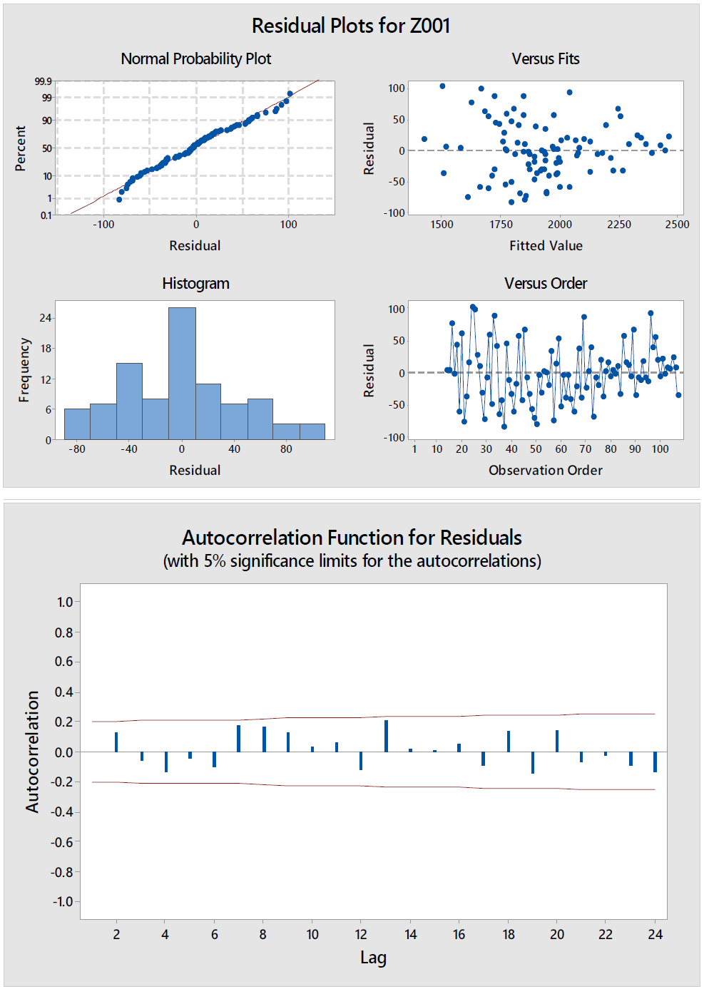
Figure 7: Residual Analysis Plots of Z001 Product

Inventory Planning Model

First step of inventory planning is to classify historical demand data into continuous demand or discrete demand. Tersine [17] proposed a method to deal with this by PETERSON-SILVER principle through calculating V value. The formulas to calculate V:

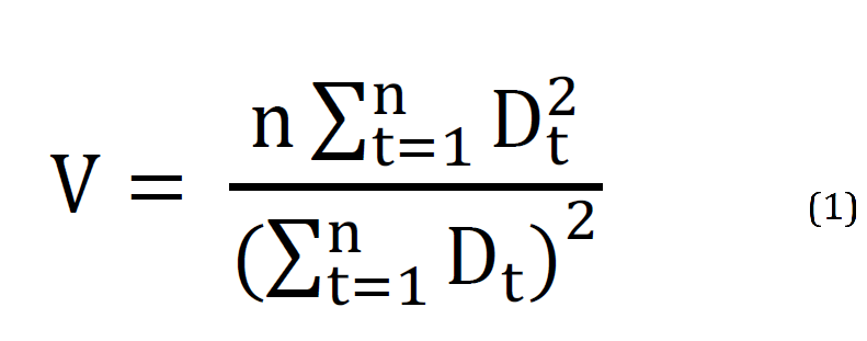
where, n is number of periods, Dt is demand per period. If V<0.25, demand has continuous pattern, else, V³0.25, demand has discrete pattern. Based on Equation 1, the products are classified as in Table 2.

Also, we can test demand pattern through 3s chart. If demand data has all value within UCL and LCL, we conclude that demand has continuous pattern. For example, with Z001 product data in Figure 8.

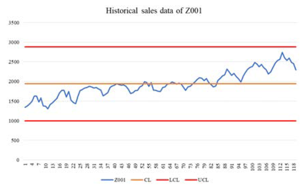
Figure 8: Six-Sigma Chart to Test Data Pattern of Z001

Table 1: Result of Applying Forecasting Techniques to Four Products

Table 2: Classification of Demand Pattern

Obviously, the demand data are between the range of upper and lower bounds, so 4 products have continuous demand patterns. Therefore, the proposed inventory model for 4 products is the Economic Production Quantity (EPQ) model. The following assumptions of EPQ model are pointed by Tersine [17]: The demand and production rate are constant and deterministic; the unit variable cost does not depend on the replenishment quantity; there are no quantity discount; the planning horizon is very long. In other words, we assume that all the parameters will continue at the same values for a long time.

Summary of the parameters and notations for the economic production quantity model of 4 products as in Table 3.

The data are collected and summarized based on company information. In EPQ model, there are 3 parameters of working stock that we should highly consider, including: Economic production quantity (Q*), reorder point (B) and total inventory cost (TC).

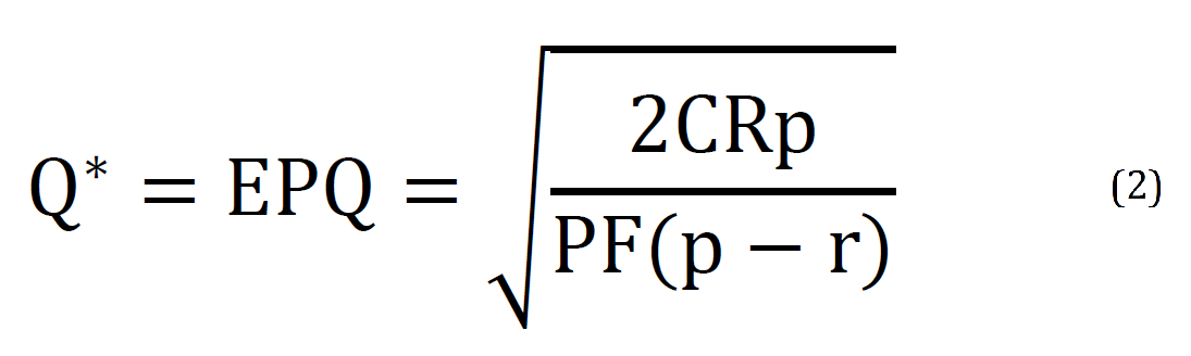
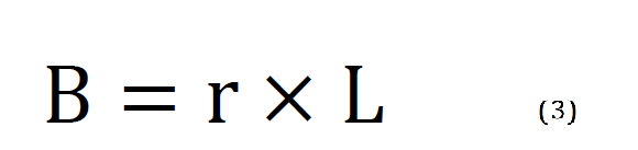
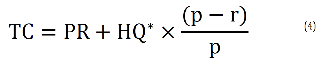
For example, applying Equation 2-4 for inventory planning for Z001 product with EPQ model, we can calculate Q* = 6,465 units, B = 574 units and TC = 55, 184, 172 VND. With the above calculation results, when the inventory level of Z001 product reaches 574 units, we should re-produce with a batch size of 6,465 units. Similar to the other products, we get the summary Table 4 of results.

Thus, the total inventory cost if using EPQ model for inventory planning is 238,700,796 VND. Besides, to deal with the risk of shortage stocks, we calculated safety stock based on forecast errors according to the formulas [18]:

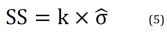
where, k is the factor of safety for achieving the target customer service level, usually calculated based on a normal distribution and is the standard deviation of the forecast error. is usually estimated by calculating the RMSE value of the forecast [18]. Therefore, we calculate the safety stock for the 4 products and the new reorder point as follows in Table 5.

Summary, in inventory planning with EPQ model, each product has working stocks (reorder point B*, production quantity Q*) and Safety Stocks (SS). Total inventory cost of 4 products, including production cost, setup cost, holding cost and safety stock cost, is 239,078,157.20 VND.

Table 3: Summary of the Parameters and Notations for the Economic Production Quantity Model

R: Demand, r: Demand rate, p: Production rate, H: Holding cost, C: Setup cost, P: Production cost, L: Leadtime

Table 4: Summary of EPQ Model for Four Products

Table 5: Summary of Calculating Safety Stock for Four Products

Table 6: Current Inventory Cost for the Z001 Product in a Year

Table 7: Inventory Costs of EPQ and Existing Policy

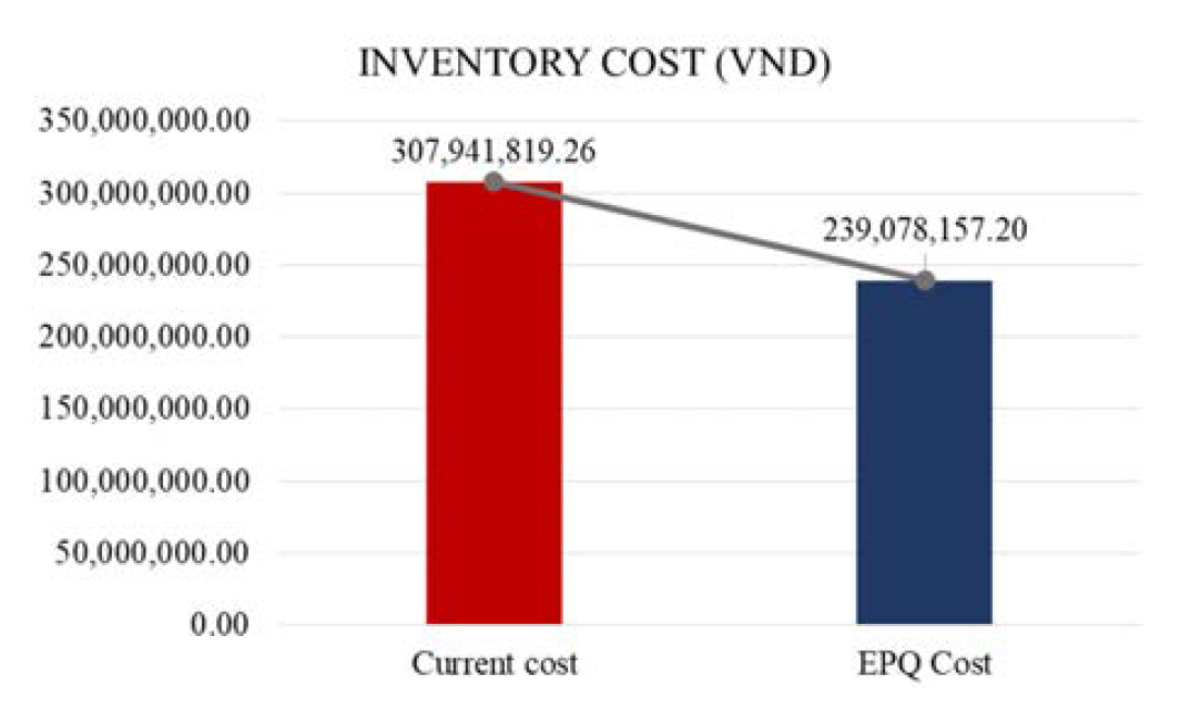
Figure 9: Comparison Between Inventory Cost of EPQ and Existing Policy

Evaluation

The company's current inventory policy is to use a certain inventory level for each product. That means the company will continuously produce to keep inventory at that certain level. For instance, estimating the current inventory cost for the Z001 product in a year as shown in the Table 6.

A similar calculation for other products. The total inventory cost of EPQ and existing policy are presented in the Table 7.

With inventory planning according to the EPQ model, the total inventory cost of 4 products reduced from VND 307,941,819.26 to VND 239,078,157, saving 22% of the total cost compared to the company's current inventory policy (Figure 9).

Our approach helps the company have an appropriate production plan and manage inventory effectively to minimize inventory costs and maximize customer service so as not to lead to serious consequences of not being able to fulfil orders for customers. The results of applying forecasting techniques and EPQ model have shown that the inventory cost decrease significantly, which saves 22% compared to inventory cost of existing policy. In summary, with the above results, our study has achieved the initial goal set out: manage customer demand through appropriate forecasting methods; reduce inventory level and decrease inventory cost but still meet customer demand.

However, in our solution, we made some assumptions to simplify problem model. This is a limitation of our study. Therefore, it is recommended that the following studies should consider assumptions that are likely to occur in reality to conduct appropriate inventory planning and apply them more closely to reality.

Acknowledgment

This research could not be completed without the effort and cooperation of our group member. We would like to express our special thanks to our research company for sharing and giving us an opportunity to implement the research at their factory. Moreover, we are grateful that company’s director and all employees always support us to complete this research. In addition, we also thank Mechanical Engineering Faculty of Hochiminh City University of Technology for providing us with financial support to complete our research.

1. Karmaker, C.L. et al. “A Study of Time Series Model for Predicting Jute Yarn Demand: Case Study.” Journal of Industrial Engineering, 2017.

2. Beutel, Anna-Lena and Stefan Minner. “Safety Stock Planning under Causal Demand Forecasting.” International Journal of Production Economics, vol. 140, no. 2, 2012, pp. 637-645.

3. Nallusamy, S. et al. “Proposed Model for Inventory Review Policy through ABC Analysis in an Automotive Manufacturing Industry.” International Journal of Engineering Research in Africa, vol. 29, 2017, pp. 165-174.

4. Lisan, Sharfuddin. “Safety Stock Determination of Uncertain Demand and Mutually Dependent Variables.” International Journal of Business and Social Research, vol. 8, no. 3, 2018, pp. 1-11.

5. Chopra, Sunil et al. “The Effect of Lead Time Uncertainty on Safety Stocks.” Decision Sciences, vol. 35, no. 1, 2004.

6. Charnes, John M. et al. “Safety Stock Determination with Serially Correlated Demand in a Periodic-Review Inventory System.” Journal of the Operational Research Society, vol. 46, no. 8, 1995, pp. 1006-1013.

7. Barrow, Devon and Nikolaos Kourentzes. “Distributions of Forecasting Errors of Forecast Combinations: Implications for Inventory Management.” International Journal of Production Economics, vol. 177, 2016, pp. 24-33.

8. Sitohang, Sunarsan and Very Karnadi. “Forecasting Method Using the Minitab Program.” Technium Social Sciences Journal, vol. 16, 2021, pp. 618-630.

9. Hanke, John E. and Dean W. Wichern. Business Forecasting. 9th ed., Pearson Education Limited, 2008.

10. Iwu, Hycinth Chukwudi et al. “Application of Inventory Model in Determining Stock Control in an Organization.” American Journal of Applied Mathematics and Statistics, vol. 2, no. 5, 2014, pp. 307-317.

11. Hossain, Md. Arafat et al. “Improved Inventory Management System for a Jute Mill: A Case Study.” Global Journal of Researches in Engineering, vol. 13, no. 10, 2013.

12. Samak-Kulkarni, Rajhans. “Determination of Optimum Inventory Model for Minimizing Total Inventory Cost.” Procedia Engineering, vol. 51, 2013, pp. 803-809.

13. Yamazaki, Tomoaki et al. “An Approach to Establishing a Method for Calculating Inventory.” International Journal of Production Research, vol. 54, no. 8, 2016, pp. 2320-2331.

14. Rizkya, I. et al. “Comparison of Periodic Review Policy and Continuous Review Policy for the Automotive Industry Inventory System.” IOP Conference Series: Materials Science and Engineering, 2017.

15. Tran Vu, Tran Thanh. Implementation of Vendor-Managed Inventory Model for Bluescope Buildings Vietnam. Master’s thesis, Ho Chi Minh City University of Technology, Vietnam National University, 2013.

16. Alam, N.M. et al. “Stochastic Model for Drought Forecasting for Bundelkhand Region in Central India.” Indian Journal of Agricultural Sciences, vol. 84, no. 1, 2014, pp. 79-84.

17. Tersine, R.J. Principles of Inventory and Materials Management. Prentice Hall, 1994.

18. Silver, Edward A. et al. Inventory and Production Management in Supply Chains. 4th ed., Taylor & Francis Group, 2017.