
+91 6002993949
submission@iarconsortium.org
Open Access
ISSN (Print) : 2708-5155
ISSN (Online) : 2708-5163
This research focused on improving the workforce scheduling problem at a plastic company. The research developed a computer program to solve two problems: shift scheduling and labor allocation, with the objective of minimizing labor costs, based on the constraints on the number of workers, the number of products, the suitability of each worker and other related constraints. The workforce scheduling program is built on the interface of MS. Excel software, VBA project and Solver, OpenSolver tool. The purpose of the program is to calculate the number of workers required for each working shift so as to optimize costs, then allocate workers to working shifts. The program was built and validated with data from the studied shop floor in 7 months. The results show that the program has arranged workers according to the corresponding shift and the speed of completing the shift schedule has been reduced by 8 times compared to the present, the total labor cost is saving average 15.1% per month. The program meets the set parameters: completion time is reduced, worker response level is increased and the time difference between shifts is less than 40%.
In this work, we studied the operation of blowing shop floors at a plastic manufacturing company in Vietnam. Because of customers’ high demand, the shop floors continuously operate 24/7. Therefore, it is extremely necessary to schedule working shifts and days off for each worker, but it’s a hard problem due to related constraints. Derived from the company's production practice and the importance of this problem, this research aims to improve the workforce scheduling problem. The research only considers data in 7 months. All data are considered in a deterministic environment, ignoring random factors such as: sudden absence of workers, urgent orders. In a 24/7 continuous work environment, managers are required to consider assigning workers to work shifts so that they do not disrupt the work cycle and to ensure optimal labor costs. Therefore, workforce scheduling is a challenging yet critical problem in both manufacturing [1,2] and services [3-5]. Workforce scheduling (human resource scheduling) deals with the arrangement of shift schedules and the assignment of workers to shifts in order to cover the demand for resources that vary over time [6]. The schedules are typically subject to various constraints dictated by equipment requirements, union rules. The resulting problems tend to be combinatorially hard. Also according to Pinedo [6], in shift scheduling-one of the problems of workforce scheduling, we consider a cycle that is fixed in advance. In certain settings the cycle may be a single day, while in others it may be a week or a number of weeks. Besides, each work assignment pattern over a cycle has its own cost and the objective is to minimize the total cost.
In the past, Hast [1] pointed out the necessary input parameters for a shift scheduling problem including: total number of current workers, the required number of workers per shift and the number of working hours per week of each worker. There were several solution models to this problem depending on their own constraints, since Barnhart et al. [7] studied formulations of integer programs with a huge number of variables and their solution by column generation methods, some approaches possibly combined with column generation were used in many other staff scheduling applications [2,8]. Specifically, as in Stark and Zimmermann [2] proposed a multi-commodity flow network for the workforce scheduling problem under consideration and show how branch-and-price can be used to solve this problem. The branch-and-price solution procedure is able to generate solutions that are on average within 10% of the lower bound in less than 20 minutes for problem instances with 50 workers.
Caprara et al. [3] proposed mathematical models and solution algorithms for a family of staff scheduling problems. Their main objective is the minimization of the number of employees needed to perform all daily assignments in the horizon, methodology is to decompose the problem into two steps: the definition of the sequence of working and rest periods for each employee and the definition of the daily assignment to be performed in each working period by each employee. Besides, some mathematical models of workforce scheduling problems were established depending on their own constraints as in [9-14]. The algorithms of these researches have contributed to the diversity of the literature review in this field.
In the next section, we focus on gathering and analyzing data to identify problems of our case study, then building a mathematical model based on literature review and presenting the research findings. For the last section, we discuss the research results and make some recommendations for the company to achieve operational efficiency.
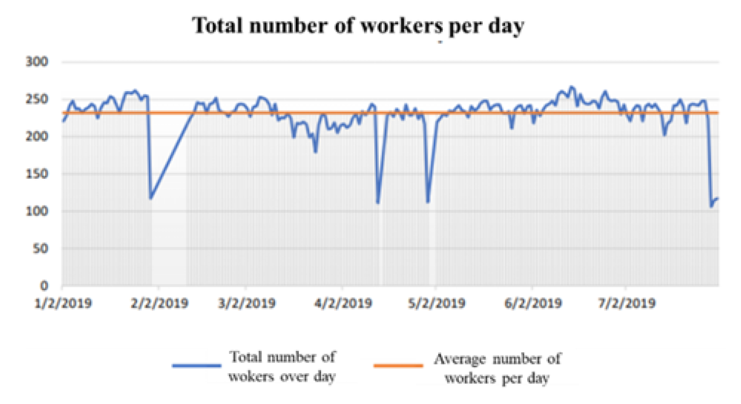
Figure 1: Total Number of Workers per Day
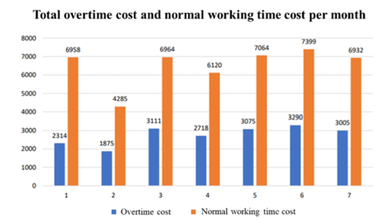
Figure 2: Total Overtime Cost and Normal Working Time Cost per Month
PROBLEM DESCRIPTION
The blowing shop floors currently operate 24/7, which makes a big problem of days-off scheduling and shift scheduling. The manager arranges to coordinate between 8-hour shifts/day and 12-hour shifts/day for all workers. The 12-hour shift includes 8 hours of normal working time and 4 hours of overtime. Overtime pay is 1.5 times an employee's normal salary per hour, which means that the more 12-hour shifts are arranged, the more labor costs will be increased. Moreover, it is necessary to balance the number of existing workers with the number of workers required from the production plan, so it’s merely important to reschedule the workforce to meet the daily required number of workers and minimize the labor costs.
The effectiveness of a workforce scheduling model was evaluated by 3 criterions: the total time of scheduling, worker response level (the level of meeting the number of workers required) and the balance rate between 8-hour shift and 12-hour shift. In fact, the manager spent around 4 hours scheduling the workforce manually at least one day in advance. However, with manual scheduling calculation, the number of workers highly varies over day (Figure 1).
Although worker response level is maintaining well because of the large number of workers, Figure 1 shows that the number of workers varies from day to day and requires a large amount of over 200 workers per day. Therefore, calculating the number of workers for each work day is necessary.
Besides, the rate between 8 hour shift and 12 hour shift is not balanced while the 12 hour shift accounts for 85% total shifts, the 8 hour shift only takes 15% the remaining one. Table 1 shows the summary of total workers per month and percentage rate of 8 hour shift and 12 hour shift.
Table 1: Total Workers in Each Shift per Month
| Month | 8 hour shift | % 8 hour shift | 12 hour shift | % 12 hour shift | Total workers |
| Jan | 2330 | 33.5% | 4628 | 66.5% | 6958 |
| Feb | 536 | 12.5% | 3749 | 87.5% | 4285 |
| Mar | 742 | 10.7% | 6222 | 89.3% | 6964 |
| Apr | 685 | 11.2% | 5435 | 88.8% | 6120 |
| May | 914 | 12.9% | 6150 | 87.1% | 7064 |
| Jun | 820 | 11.1% | 6579 | 88.9% | 7399 |
| Jul | 922 | 13.3% | 6010 | 86.7% | 6932 |
| Total | 6949 | 15.2% | 38773 | 84.8% | 45722 |
The unbalanced rate between the 8 hour shift and the 12 hour shift causes the high labor cost at the shop floor, where overtime pay is 1.5 times an employee's normal salary per hour. As a result, the cost of overtime is currently very large, accounting for nearly 40% of the total labor cost, which leads to the high labor cost (Figure 2).
Generally, the company’s workforce scheduling method needs optimizing time and labor cost but still meets the production plan requirement. This research focuses on generic workforce scheduling problems, including shift scheduling and labor allocation, then develops a computer program to support the company's leader.
Mathematical Model
There are some fixed constraints of workforce scheduling problem at shop floor:
Model 1: Shift Scheduling Problem
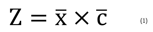
According to Pinedo [6], the problem can be formulated in matrix type as follows.
Objective
Minimize:
Constraints
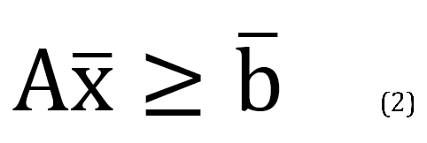
where, i is the index of time period (i = 1, 2,…, m); j is the index of working shift (j = 1, 2,..., n); aij is the binary variable, aij = 1 if period i is a work period and 0 otherwise; bi is number of workers required from the production plan; cj is the cost of assigning a worker to shift j; xj is the decision variable representing the number of workers assigned to shift j; A is the matrix of aij and ![]() ;
; ![]() ;
; ![]() is the vector of xj; cj; bi.
is the vector of xj; cj; bi.
Model 2: Labor Allocation Problem
Output of model 1 (shift scheduling) is the number of workers for each working shift in a day, this will be the input model 2 (labor allocation). The objective of model 2 is to find a schedule for each worker including their days off, working days, working shifts in order to minimize total labor cost. In particular, it is necessary to consider the skills and suitability of workers for the types of products from the production plan.
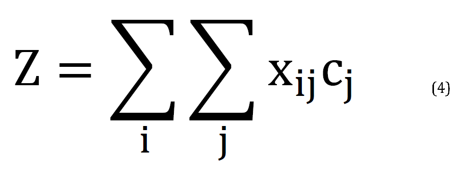
Objective
Minimize:
Constraints
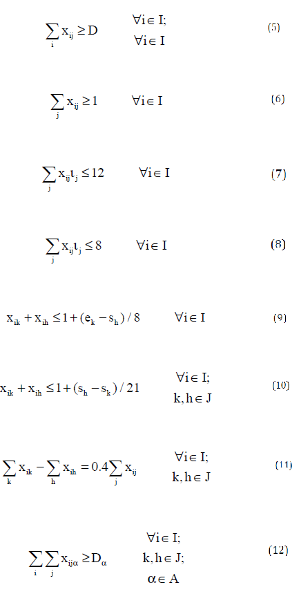
where, I is the set of workers; J is the set of working shifts; lj is the time of shift j (length of shift j); sj is the start time of the shift j; ej is the end time of the shift j; D is the number of workers required from the production plan, A is the set of products with high quality requirements; c is the normal working time labor cost per hour (1.5c: overtime labor cost per hour); xij is the decision variable (binary variable), xij = 1 if worker i is assigned to shift j, otherwise xij = 0 and Da: number of workers required for a-type product.
The objective function (4) is to minimize the total labor cost in the working shifts. Constraint (5) ensures that the number of workers working in a day meets the number of workers needed that day. Constraint (6) shows that each worker can only work 1 shift per day. Constraint (7) and (8) show that the maximum and minimum time of a working shift are 12 hours and 8 hours. Constraint (9) demonstrates the time between 2 shifts of 1 worker is at least 8 hours, similarly, constraint (10) is about that the time of day-off is at least 21 hours (the time between start time and end time of day-off). Constraint (11) shows that the difference between 12-hour shift and 8-hour shift is less than or equal to 40%. Last, constraint (12) is a hard constraint, workers are assigned to shift with appropriate skills.
Data Collection
Level of products, level of workers and number of workers required for each product: The blowing shop floor currently produces 310 products and has 260 workers. Because of the company’s private policy, products and workers are encoded: SP001, SP002,…, SP310 (products) and CN001, CN002,…, CN260 (workers). Products are divided into 4 levels based on their difficulties. Correspondingly, workers are also divided into 4 levels depending on their skills. 4-level workers can make all products of 4 levels. 3-level workers can make products of level 3 or below. Similarly, 2-level workers can make products of level 1 and level 2. 1-level workers are only arranged to make products of level 1. Besides, each product requires a certain number of workers. These were shown in Table 2-4.
Table 2: Number of Workers Required for Each Products
Product | Number of workers required |
SP001 | 3 |
SP002 | 3 |
SP003 | 3 |
… | … |
SP309 | 1 |
SP310 | 1 |
Table 3: Level of Each Worker
Worker | Level of Worker | |||
1 | 2 | 3 | 4 | |
CN001 | X | |||
CN002 | X | |||
CN003 | X | |||
… | … | … | … | … |
CN259 |
|
| X |
|
CN260 |
|
| X |
|
Table 4: Level of Each Product
Product | Level of Product | |||
1 | 2 | 3 | 4 | |
SP001 | X | |||
SP002 | X | |||
SP003 | X | |||
… | … | … | … | … |
SP309 |
| X |
|
|
SP310 |
| X |
|
|
Matrix A(m,n): Divide each day into 24 intervals of 1 hour. In fact, the blowing workshop divides the working shift of 12 hours/day and 8 hours/day, so each day can be divided into 2 shifts of 12 hours and 3 shifts of 8 hours. The detailed information of working shifts are shown in Table 5, then matrix A(m,n) is built as Table 6.
Labor cost unit: With the assumption of normal working time cost is 20,000 VND/hour, the overtime cost is 1.5 times and the night working cost is 1.2 times normal working time cost. Table 7 demonstrates the summary of labor cost of each shift.
Table 5: Information of Working Shifts
| Shift (S1) | Shift (S2) | Shift (S3) | Shift (S4) | Shift (S5) |
Length of shift | 12 hour | 12 hour | 8 hour | 8 hour | 8 hour |
Start time | 6 am | 6 pm | 8 am | 4 pm | 12 Am |
End time | 6 pm | 6 am | 4 pm | 12 am | 8 Am |
Table 6: Matrix A (m,n)
| Time interval | Shift (S1) | Shift (S2) | Shift (S3) | Shift (S4) | Shift (S5) |
6-7 | 1 | 1 | |||
7-8 | 1 | 1 | |||
8-9 | 1 | 1 | |||
9-10 | 1 | 1 | |||
10-11 | 1 | 1 | |||
11-12 | 1 | 1 | |||
12-13 | 1 | 1 | |||
13-14 | 1 | 1 | |||
14-15 | 1 | 1 | |||
15-16 | 1 | 1 | |||
16-17 | 1 | 1 | |||
17-18 | 1 | 1 | |||
18-19 | 1 | 1 | |||
19-20 | 1 | 1 | |||
20-21 | 1 | 1 | |||
21-22 | 1 | 1 | |||
22-23 | 1 | 1 | |||
23-0 | 1 | 1 | |||
0-1 | 1 | 1 | |||
1-2 | 1 | 1 | |||
2-3 | 1 | 1 | |||
3-4 | 1 | 1 | |||
4-5 | 1 | 1 | |||
5-6 | 1 | 1 |
Table 7: Summary of Labor Cost for Each Shift
Shift | S1 | S2 | S3 | S4 | S5 |
Labor cost (kVND/worker) | 280 | 312 | 160 | 184 | 184 |
The workforce scheduling program is built on the interface of MS. Excel software, VBA project and Solver, OpenSolver tool. Running 2 mathematical models, the results were demonstrated in this sections.
Shift Scheduling
Based on the required number of workers per day, then run the shift scheduling program to calculate the number of workers working in each shift. With the number of workers required for each hour is 100 workers/hour, the solving speed of the program is 2 minutes/time. Table 8 shows the result of the shift scheduling program for the first 14 days of July.
Due to the constraint that the total number of workers in the 12 hour shift must be larger than in the 8 hour shift (the company's policy to ensure wages for workers), the program calculates that the number of workers in the 12 hour shift is larger than in the 8 hour shift, but still ensure optimal labor costs.
Based on the results of the workforce scheduling program shown in Table 9, compared to the company's data shown in Table 10, the workforce scheduling program is much more optimal. The unbalanced rate between 8 hour shift and 12 hour shift has improved a lot and still ensures the required number of workers per day (Figure 3). On July 1, with a total required worker of 102 people/hour, the program calculated that the total number of workers working in the 12 hour shift was 124 people and the 8-hour shift was 120 people, a difference of 2%. Meanwhile, the manual shift has quite a large difference, the total number of workers in the 8-hour shift is only 17 people while in the 12 hour shift, it is up to 226 people, similar to other days.
Labor Allocation
Running the labor allocation program can specifically arrange which workers work in which shifts per day. The program runs with 1300 binary variables (aij), the solving speed is about 5 minutes/time. For example with the data of July 1st 2019, the number of workers required is 102 workers/hour, the result from shift scheduling program is 120 workers working the 8-hour shift and 124 workers working the 12 hour shift ( detailed in previous section), the results of the labor allocation program are shown in Figure 4, corresponding to the result of the shift scheduling program.
Table 8: Shift Scheduling Result
Date | 1-Jul | 2-Jul | 3-Jul | 4-Jul | 5-Jul | 6-Jul | 7-Jul | 8-Jul | 9-Jul | 10-Jul | 11-Jul | 12-Jul | 13-Jul | 14-Jul |
No. of workers required | 102 | 96 | 92 | 98 | 101 | 101 | 92 | 101 | 102 | 100 | 102 | 98 | 97 | 85 |
(S1) | 62 | 58 | 56 | 59 | 61 | 61 | 56 | 61 | 62 | 60 | 62 | 59 | 59 | 57 |
(S2) | 62 | 58 | 56 | 59 | 61 | 61 | 56 | 61 | 62 | 60 | 62 | 59 | 59 | 57 |
(S3) | 40 | 38 | 36 | 39 | 40 | 40 | 36 | 40 | 40 | 40 | 40 | 39 | 38 | 38 |
(S4) | 40 | 38 | 36 | 39 | 40 | 40 | 36 | 40 | 40 | 40 | 40 | 39 | 38 | 38 |
(S5) | 40 | 38 | 36 | 39 | 40 | 40 | 36 | 40 | 40 | 40 | 40 | 39 | 38 | 38 |
Table 9: Total workers of each shift per day using shift scheduling program
Date | 8 hour shift (S3+S4+S5) | 12 hour shift (S1+S2) | % 8 hour shift | % 12 hour shift |
1-Jul | 120 | 124 | 49% | 51% |
2-Jul | 114 | 116 | 50% | 50% |
3-Jul | 108 | 112 | 49% | 51% |
4-Jul | 117 | 118 | 50% | 50% |
5-Jul | 120 | 122 | 50% | 50% |
6-Jul | 120 | 122 | 50% | 50% |
7-Jul | 108 | 112 | 49% | 51% |
8-Jul | 120 | 122 | 50% | 50% |
9-Jul | 120 | 124 | 49% | 51% |
10-Jul | 120 | 120 | 50% | 50% |
11-Jul | 120 | 124 | 49% | 51% |
12-Jul | 117 | 118 | 50% | 50% |
13-Jul | 114 | 118 | 49% | 51% |
14-Jul | 114 | 114 | 50% | 50% |
Table 10: Total workers of each shift per day using manual method (current stage)
Date | 8-hour shift (S3 + S4 + S5) | 12-hour shift (S1 + S2) | % 8-hour shift | % 12-hour shift |
1-Jul | 17 | 226 | 7% | 93% |
2-Jul | 14 | 215 | 6% | 94% |
3-Jul | 23 | 198 | 10% | 90% |
4-Jul | 24 | 212 | 10% | 90% |
5-Jul | 19 | 223 | 8% | 92% |
6-Jul | 15 | 226 | 6% | 94% |
7-Jul | 6 | 215 | 3% | 97% |
8-Jul | 130 | 111 | 54% | 46% |
9-Jul | 19 | 225 | 8% | 92% |
10-Jul | 25 | 214 | 10% | 90% |
11-Jul | 23 | 221 | 9% | 91% |
12-Jul | 29 | 208 | 12% | 88% |
13-Jul | 28 | 203 | 12% | 88% |
14-Jul | 11 | 191 | 5% | 95% |
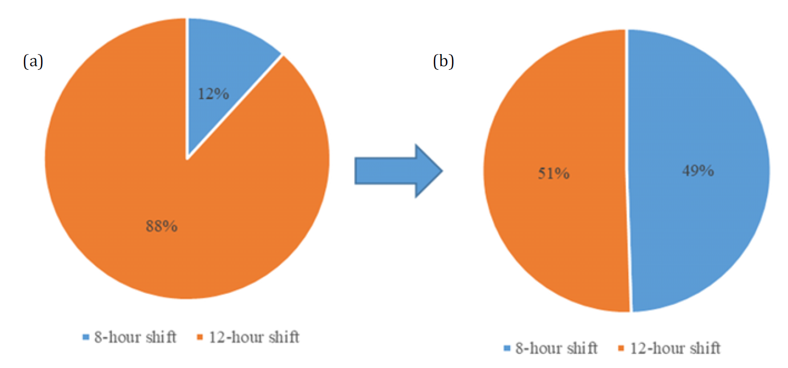
Figure3(a-b): The Different Rate of Shifts Before and After Improving, (a) Manual Scheduling Method and (b) Workforce Scheduling Method
Labor Cost
Total labor cost calculated by workforce scheduling program and manual method are shown in Table 11.
Apparently, total labor cost using workforce scheduling program is more optimal thanmanual scheduling due to the balanced rate between 8 hour shift and 12 hour shift. The average saving rate of labor cost is 15.1%.
As mentioned before, there are 3 criterions to evaluate the workforce scheduling model: the total time of scheduling, the level of meeting the number of workers required and the balance rate between 8 hour shift and 12 hour shift.
For the first criterion, the total time of scheduling has been reduced much lower than the actual stage. Currently, the manager spent around 4 hours scheduling the workforce manually. When using our model, it takes about 10 minutes to run the program from entering the production plan until the shift allocation table is produced. Including the time to be considered and adjusted by the shift leader, it only takes about 30 minutes to arrange the next day's shift. The model calculates the optimal cost of allocating workers, but still ensures that the number of workers is always greater than or equal to the required number of the production plan. For the last criterion, the unbalanced percentage rate has been greatly reduced as shown in the result section. The rate between 8-hour shifts and 12 hour shifts is only about 10-20%, but still ensures the number of workers required.
The company is growing, the manual workforce scheduling model is no longer effective. Therefore, application of this new workforce scheduling model is necessary and completely suitable with the current conditions. Workforce scheduling research at a plastic company with shift scheduling model and labor allocation model gives optimal results, which is more efficient than the current method. However, the research only considers deterministic conditions, ignoring unexpected factors, so when operating the model, it is necessary to consider and be evaluated by the shift leader. In the future, we recommend expanding the related research on workforce scheduling problems considering more random factors. Moreover, it’s considerable to develop a computer program for workforce scheduling, which helps users easily access and store information.
Table 11: Total Labor Cost Using Workforce Scheduling Program and Manual Method
Date | Workforce scheduling program | Manual scheduling |
1-Jul | 57,824,000 | 69,880,000 |
2-Jul | 54,400,000 | 66,112,000 |
3-Jul | 52,160,000 | 62,648,000 |
4-Jul | 55,520,000 | 66,976,000 |
5-Jul | 57,232,000 | 69,352,000 |
6-Jul | 57,232,000 | 69,536,000 |
7-Jul | 52,160,000 | 64,680,000 |
8-Jul | 57,232,000 | 55,704,000 |
9-Jul | 57,824,000 | 69,912,000 |
10-Jul | 56,640,000 | 67,728,000 |
11-Jul | 57,824,000 | 69,440,000 |
12-Jul | 55,520,000 | 66,664,000 |
13-Jul | 54,992,000 | 64,984,000 |
14-Jul | 53,808,000 | 58,448,000 |
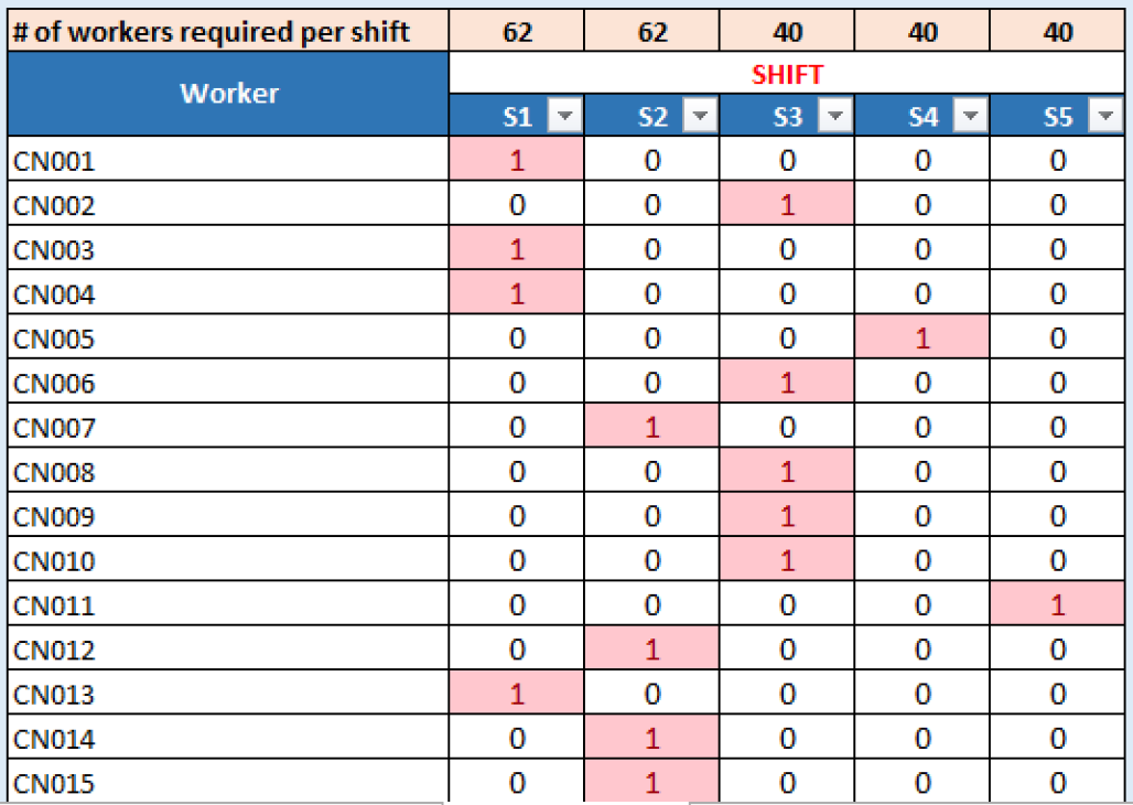
Figure4: Labor Allocation Result
Acknowledgment
We are grateful to the company for sharing and giving us an opportunity to implement the improvement.
Hast, J. Optimal Work Shift Scheduling: A Heuristic Approach. Master’s Programme in Mathematics and Operations Research, Aalto University, 2017.
Stark, C. and J. Zimmermann. “An Exact Branch-and-Price Algorithm for Workforce Scheduling.” Operations Research Proceedings, vol. 2004, Springer, 2004, pp. 207-212.
Caprara, A. et al. “Models and Algorithms for a Staff Scheduling Problem.” Mathematical Programming, Series B, vol. 98, 2003, pp. 445-476.
Talbot, F.B. and James H. Patterson. “An Efficient Integer Programming Algorithm with Network Cuts for Solving Resource-Constrained Scheduling Problems.” Management Science, vol. 24, no. 11, 1978, pp. 1163-1174.
Millar, H.H. and M. Kiragu. “Cyclic and Non-Cyclic Scheduling of 12h Shift Nurses by Network Programming.” European Journal of Operational Research, vol. 104, 1998, pp. 582-592.
Pinedo, M.L. Planning and Scheduling in Manufacturing and Services. Springer, New York, 2009.
Barnhart, C. et al. “Branch-and-Price: Column Generation for Solving Huge Integer Programs.” Operations Research, vol. 46, 1998, pp. 316-329.
Mehrotra, A. et al. “Optimal Shift Scheduling: A Branch-and-Price Approach.” Naval Research Logistics, vol. 47, 2000, pp. 185-200.
Aykin, T. “A Comparative Evaluation of Modeling Approaches to the Labor Shift Scheduling Problem.” European Journal of Operational Research, vol. 125, 2000, pp. 381-397.
Billionnet, A. “Integer Programming to Schedule a Hierarchical Workforce with Variable Demands.” European Journal of Operational Research, vol. 114, 1999, pp. 105-114.
Jaumard, B. et al. “A Generalized Linear Programming Model for Nurse Scheduling.” European Journal of Operational Research, vol. 107, 1998, pp. 1-18.
Brusco, M.J. and L.W. Jacobs. “Personnel Tour Scheduling When Starting-Time Restrictions Are Present.” Management Science, vol. 44, 1998, pp. 534-547.
Thompson, G.M. “Labor Staffing and Scheduling Models for Controlling Service Levels.” Naval Research Logistics, vol. 44, 1997, pp. 719-740.
Beaumont, N. “Scheduling Staff Using Mixed Integer Programming.” European Journal of Operational Research, vol. 98, 1997, pp. 473-484.