Audio band is within the frequency range of 20Hz and 20KHz. This means that any signal between this range can be heard by humans [1].

        However, audio wave cannot travel a far distance because of attenuation. Attenuation is the loss in signal strength as it travels form one location to another. Attenuation is represented in decibels (dB), which is ten times the logarithm of the signal power at a particular input divided by the signal at an output of a specified medium.(CAS DATA LOGGERS,n.d.).

        The higher the frequency of a signal, the farther it can travel and vice versa. Thus, for an audio signal to be able to travel far, it must be modulated.

        This work will be viewed under the following objectives:

Objectives

• To determine the frequency at the centre of my voice in the MATLAB IDE

• To produce a modulated frequency with my voice using a chosen a carrier frequency in the MATLAB IDE

• To demodulate the modulated signal in order to recover back a sine wave( i.e the frequency of my voice) in the MATLAB IDE

Theory 

Modulation: Modulation is the process of modifying some parameters of a CARRIER SIGNAL with the aid of a lower frequency-MODULATING SIGNAL. The message signal to be transmitted is the modulating signal. When a signal is modulated, its frequency characteristics are modified to match a certain purpose. Types of modulation is basically categorised into two depending on whether the technology employed is analogue or digital. The two categories are: 

• Analogue modulation

• Digital modulation

Analogue Modulation Types

• Amplitude Modulation (AM): is a process where the amplitude (voltage) applied to the carrier is varied over time

• Frequency Modulation (FM): is a process where the frequency of the carrier waveform is made to change in a meaningful amount depending on the frequency of the modulating signal

• Phase Modulation (PM): is a process where the natural flow of the periodic sinusoidal signal is delayed temporarily

The above analogue modulation can also be called continuous modulation [2].

Digital Modulation Types

• Phase Shift Keying (PSK): this describes the modulation technique used to alter the phase of a carrier

• Frequency Shift Keying (FSK): this describes the technique used in the modulation of a carrier which results in a frequency for a logic 1 and a different frequency for a logic 0

• Amplitude Shift Keying (ASK): it involves the modulation technique used to multiply the carrier wave by the digital signal

Reasons for Modulation 

• It enhances easy radiation and reception of signals

• It affords the use of practically realisable antenna sizes

• It allows for channel assignment. That is, each message signal can be assigned a unique frequency band within the area of operation

• It reduces noise and interference

• It allows multiplexing of several messages over a single channel [2]

Am Modulation

Because AM modulation is used in this literature for audio signal to be transmitted, more emphasis will be laid on it.

In AM modulation, the information signal which is the modulating frequency varies the amplitude of the carrier sine wave. Thus, the amplitude of the carrier frequency changes in accordance with the variation in amplitude and frequency of the modulating signal. The frequency of the carrier waveform remains constant, but its amplitude changes in accordance with the amplitude of the modulating signal. Increase in the amplitude of the modulating signal causes a corresponding increase in the peak of the carrier frequency and vice versa.

AM is used in sound broadcasting(medium wave and short wave), in television(picture transmission), in telephony, etc.

The following is a list of some types of amplitude modulation:

• DSB (double sideband full- carrier) AM

• DSB (double sideband suppressed- carrier) AM

• SSB-RC (single sideband reduced-carrier) AM

• SSB-SC(single side band suppressed-carrier) AM

• Vestigial sideband TV

• Independent-sideband emission etc [2]

During modulation of AM signal, up to two-third of the transmitted power is in the carrier which does not carry any information. To improve the efficiency of amplitude modulation, the carrier wave must be suppressed. 

If the carrier is suppressed the two side bands remaining, we have: Double side band suppressed carrier ( popularly called DSSC or DSB).

To better improve the efficiency of modulation, one sideband can be eliminated after the carrier is suppressed. This is called single side band full carrier ( SSB-FC).

In this assignment double side band (DSB-FC) was employed.

Construction of AM wave

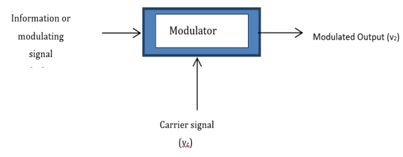
An amplitude-modulated wave is obtained by superimposing modulating signal on the carrier signal as diagrammatically shown in Figure 1 below:

v₂ = V_csin 2f_ct+ (V_m sin 2f_mt)(sin 2f_ct)

Carrier wave can be expressed with the following mathematical expression: 

v_c = V_c sin 2f_ct

(1)

• v_c= instantaneous value of the carrier sine wave voltage at some specific time in the circle

• V_c= peak value of the constant unmodulatedcarrier sine wave as measured between zero and the maximum amplitude of eitherthe positive-going or the negative-going alternation

Figure 1: Modulation of Signal

Where

 V_c = V_(p-p)

• f_c = frequency of carrier sine wave

• t = a point in time during the carrier cycle

Also, the modulating signal can be expressed with the following mathematical 

Expression:

v_m = V_m sin 2f_mt

(2)

• v_m= instantaneous value of information signal.

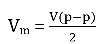
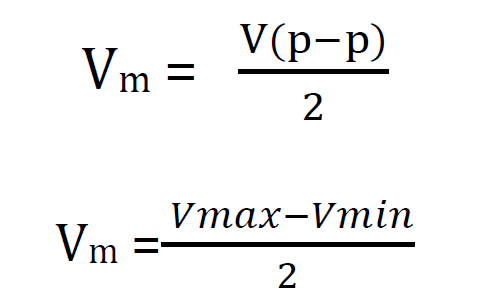
• V_m= peak amplitude of information signal, where 

• F_m = frequency of carrier sine wave

• t = a point in time during the information signal cycle

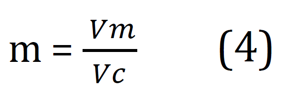
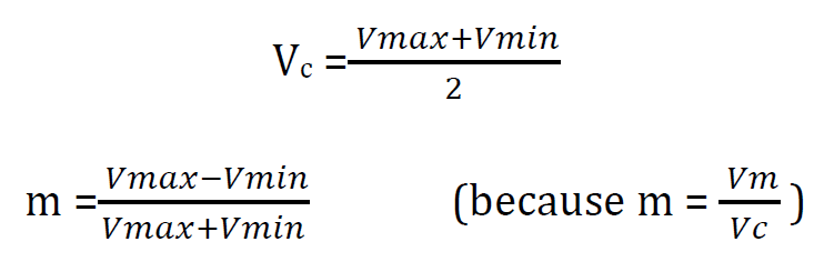
The degree of superimposition of modulating signal on the carrier signal is measured by the MODULATION DEPTH, m, of the AM wave. Modulation depth can be defined as the ratio of amplitude of modulating signal to the carrier signal amplitude. It can be expressed in percentage. Then modulation depth is Modulation Percentage(m%).

• If m > 1 we’ve over modulation

• If m = 1 we’ve critical modulation

• If m < 1 we’ve under modulation

In percentage, we’ve:

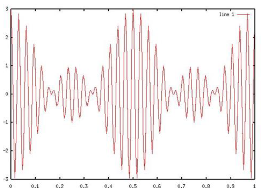
In practice, the modulating percentage of an AM signal is never allowed to reach 100% or above. If this happens recovering the information will be almost impossible with a simple circuit. If modulation percentage exceeds 100%, this is called OVER-MODULATION [2]. 

To avoid distortion of modulated signal, it is important that the peak value of the modulating signal be less than the peak value of the carrier. Mathematically, 

V_m<V_c

From the knowledge that the peak value of the carrier is the reference point for the modulating signal (i.e. the zero reference line of the modulating signal coincides with the peak value of unmodulated carrier), Formula to express the complete modulated wave is as derived below:

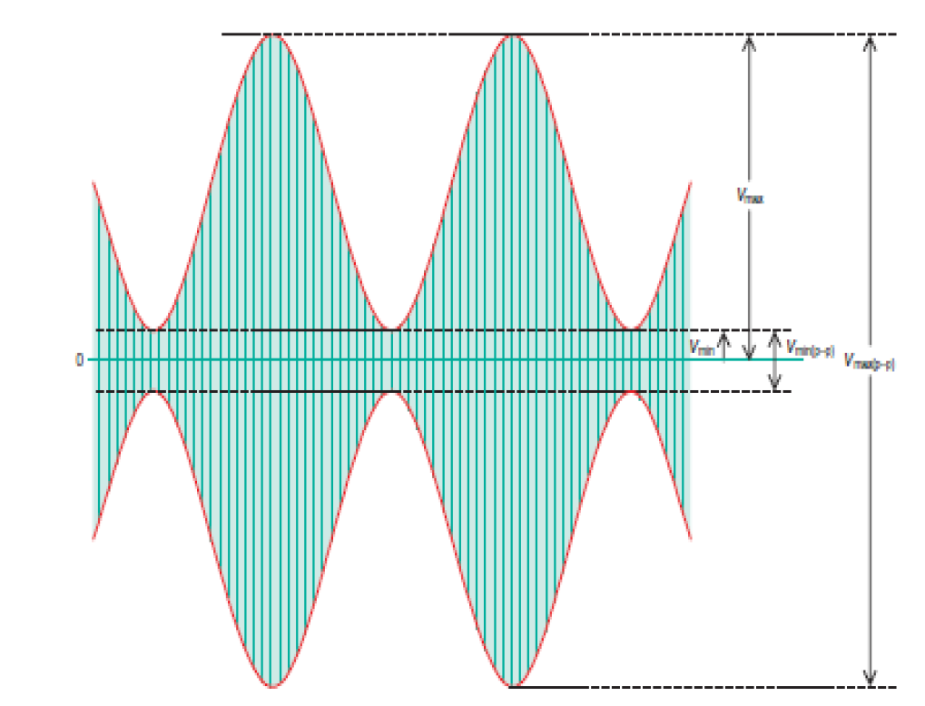
As shown in Figure 2-3 below, the instantaneous value of either the top or the bottom voltage envelope v₁ can be computed by using the following equation:

v₁ =V_c + v_{m =} V_c + V_m sin 2f_m

(6)

The above equation expresses the fact that the instantaneous value of the modulating signal algebraically adds to the peak carrier. The instantaneous value of the complete modulated wave v₂ can be written like as given below:

v₂ = v₁ sin 2f_ct

(7)

v₂ = (V_c+ V_m sin 2f_mt)sin 2f_ct

(7.1)

v₂ = V_csin 2f_ct+ (V_m sin 2f_mt)(sin 2f_ct),

Where

• v₂ is the instantaneous value of the AM wave

• V_csin 2f_ct is the carrier waveform

• (V_m sin 2f_mt)(sin2f_ct) is the product of carrier frequency and modulating frequency

• Amplitude modulation showing input and output

Where 

Figure 2: AM modulation of signals (Data Communications, n.d.)

Figure 3: Illustrating Over-Modulation

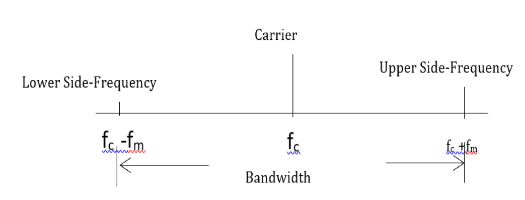
Figure 4: AM Spectrum

AM spectrum and Bandwidth

A simple AM signal contains three frequency components:

• The carrier frequency, f_m

• The lower side-frequency, f_c - f_m

• the upperside-frequency, f_{c +}f_m

Frequencies f_c and f_m are carrier carrier and modulating frequencies respectively.

As shown above, the two side frequencies contain the original message information. The two side-frequency-components have equal amplitude which is much smaller than the amplitude of the carrier frequency. This requires more power for transmission even though it has no message information.

For the transmission of AM signal whose spectrum is shown above, the two side frequencies must be given because if not, message will be lost. TRANSMISSION BANDWIDTH, B, is

B = (f_c +f_m) – (f_c - f_m) = 2 f_m

Power Distribution in the AM Waveform

The total effective (rms) power, P_Tin the AM wave is the addition of effective carrier power level, P_c and the effective sideband power levels, P_LSB and P_USB. i.e. 

P_T=P_c +P_LSB+P_USB

(8)

= V²_c(rms)/R + V²_LSB(rms)/R + V²_USB(rms)/R

(8.1)

= (0.707 V_c)²/R + ( 0.707V_LSB)²/R + (0.707 V_USB)²/R

(8.2)

= V_c²/2R + V_LSB²/2R + V_USB²/2R

(8.3)

Since power in the upper sideband is equal to power in the lower sideband                          And putting V_m = mV_c into equation 8.2

We’ve:     

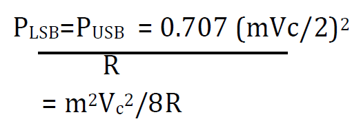
Because total power P_cin the carrier is, V_c²/2R, we’ve:

We’ve:     P_LSB= P_USB = m²Pc/4

(8.4)

FromP_T = P_LSB+ P_USB+ P_c 

We’ve: P_T = m²Pc/4 + m²Pc/4 + Pc

P_T = Pc (m²/4 + m²/4 + 1)

= Pc (m²/2 +1)

(8.5)

Power Distribution in AM Transmission for 100% Modulation

P_T = P_c (1²/2 + 1)

P_T = 1.5 P_c

(8.6)

Conclusion

• Following what we have in equation 8-4 above, if one is transmitting only one sideband of the 100% modulation, one-quarter of the effective power consumed by the carrier is used in transmission

• If it is two sidebands of the 100% modulation is being transmitted, one and a half of the effective power consumed by the carrier is used in transmission

• If carrier is suppressed, total effective power used in transmission of the 100% modulation AM signal is a lot reduced(i.e 1.5/P_c )

To Determine the Frequency at the Centre of my Voice in the MATLAB IDE

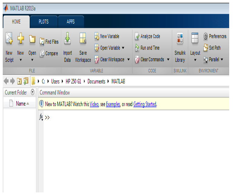
Matlab was loaded from the ‘start menu’ of the system and the window below came up:

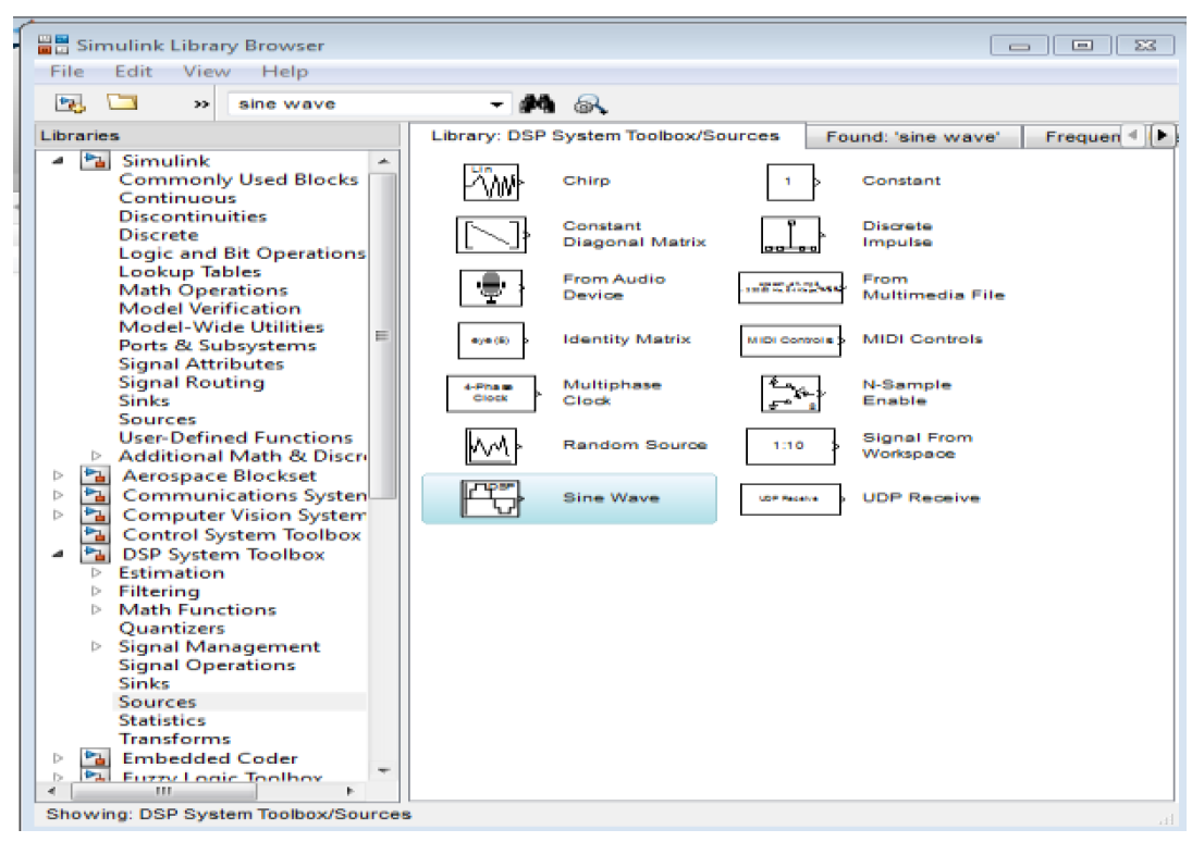
The Simulink icon in MATLAB task bar was clicked upon and ‘Simulink Library Browser’ came up as shown below:

Figure 5: Matlab IDE

Figure 6: Simulink Library Browser

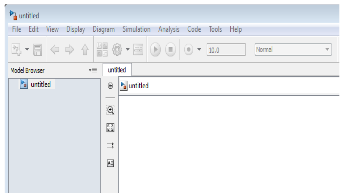
Figure 7: Model Window

Figure 8: Model Window Showing Procedure to Save File

Figure 9: Simulation of my Voice

From the Simulink library browser, ‘File’ followed by ‘New’ followed by ‘Model’ were clicked upon and a GUI work space came up as shown (Figure 6).

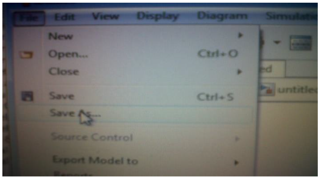
From the Simulink Model Window, ‘File’ was clicked upon followed by ‘Save As’ as shown above and this work was saved as ‘my voice.mdl’ on the desktop. From the ‘Simulink Library Browser’, ‘DSP System Tool Box’ was clicked upon followed by the ‘Sources.’ Then ‘From Audio Device’ block was dragged and dropped in ‘model window.’

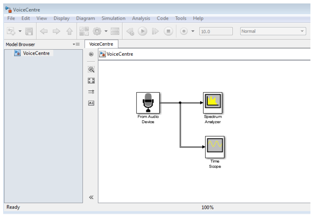
From the ‘Simulink Library Browser’ again, ‘DSP System Tool Box’ was clicked upon again then after the ‘Sinks’ and ‘Time Scope’ was dragged and dropped in the Model Window. Both ‘From Audio Device’and’ Time Scope’ blocks were connected together as shown in the Figure 8.

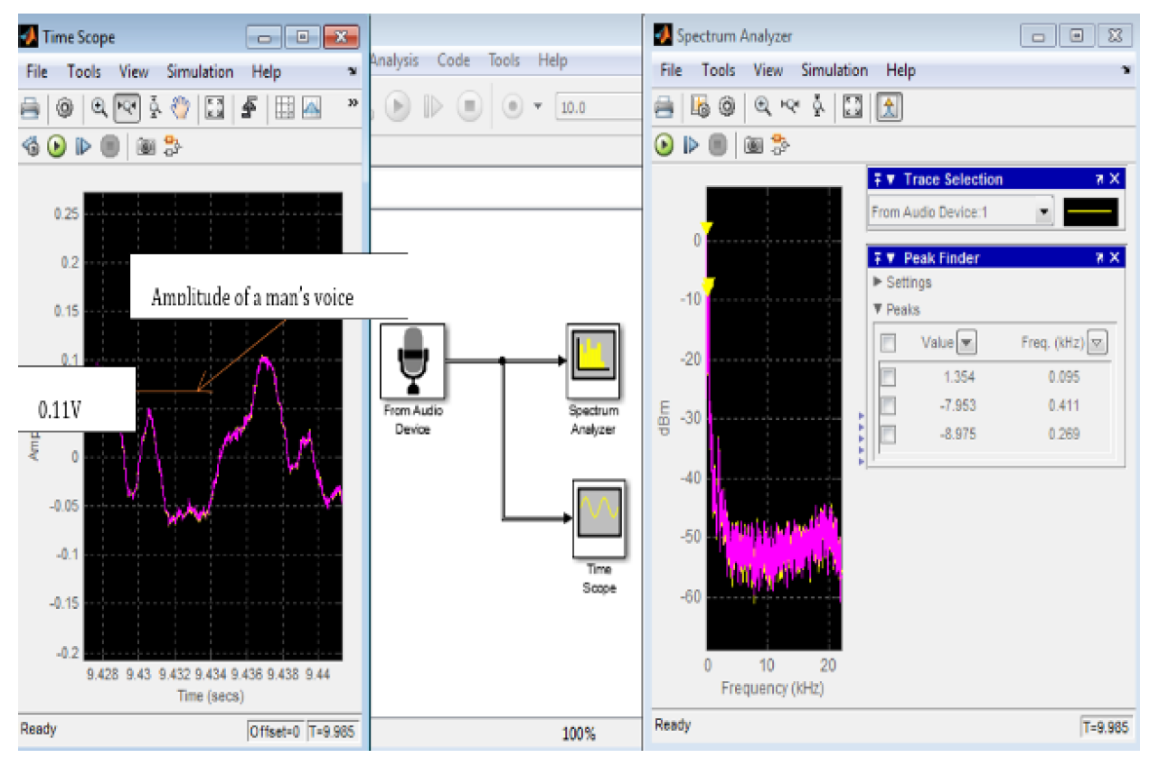
Then earpiece was connected to the PC in which there was the setup shown in Figure 9 and the simulation was run. The result shown in Figure 10 below came up.

From the Time Scope shown above, amplitude of man’s voice is 0.11V Figure 11.

Conclusion

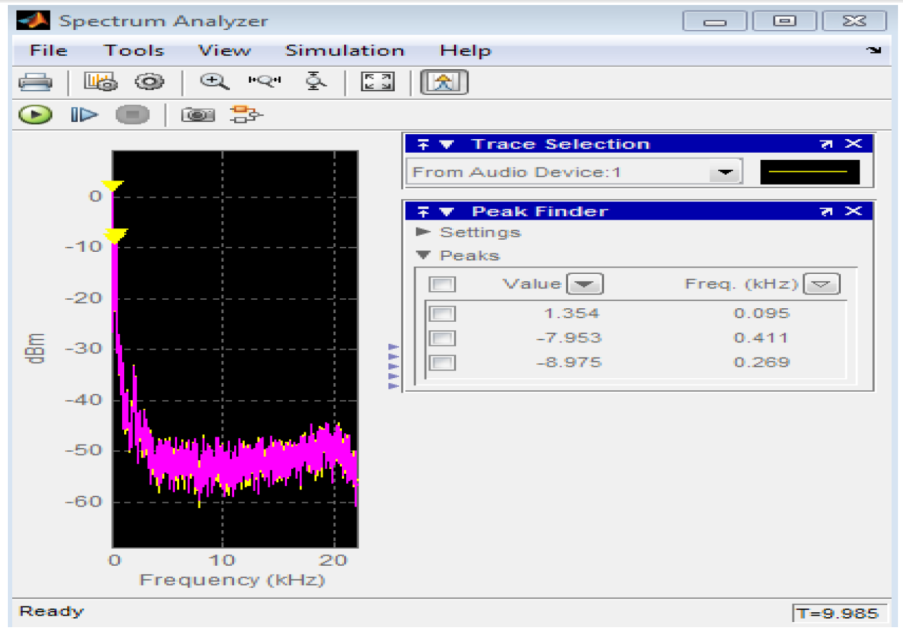
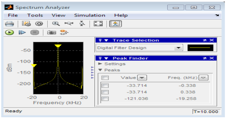
From the frequency spectrum of a man’s voice as shown in figure6 above and peak finder shown in figure7 above, the fundamental frequency of the man’s voice is found to be 411Hz and its highest harmonic 269Hz

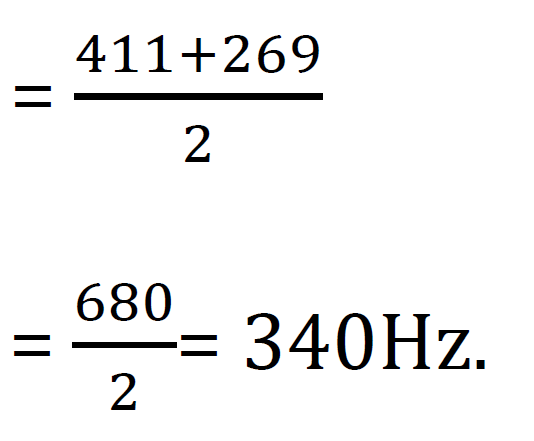
Frequency at the centre of my voice range = average of the two frequencies given above

Figure 10: Showing Frequency Spectrum of Man’s Voice

Figure 11: Peak Finder Showing the Peak Frequencies of a Man’s Voice

To produce a modulated frequency with my voice using a chosen a carrier frequency in the 

Matlab Ide

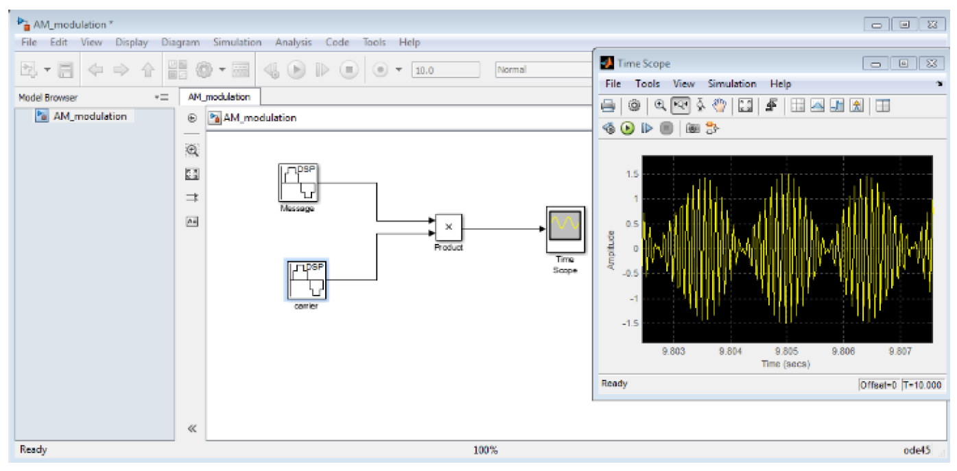
A new ‘Model Environment’ in the MPLAB IDE was opened. The procedure followed in the production of a man’s voice as described above was repeated but this time ‘Sine Wave’ block, ‘product ’ block and ‘Time Scope’ block were connected together as shown in figure8 below. The parameters of the message and carrier blocks were set as follows:

Message

• Frequency 340Hz (fundamental frequency of my voice as produced in figure6 above) 

• Amplitude modulated signal was0.11V

• F = 1/T, i.e. Sampling frequency Fs = 40000Hz

• Fs> 2(Fc + BW), where BW is the original modulated signal bandwidth.

• BW = 2fm = 2 x 340 = 680Hz 

• Fc = 9800Hz 

• Fs> 2( 9800 + 680)

• Fs> 2 (10480)

• Fs> 20960(meaning Fs must be greater than 20,928Hz) 

• So, choosing Fs = 40000Hz is justified (Mathworks, n.d.)

Carrier 

• Frequency chosen carrier frequency is 9800Hz because it must be higher than the information signal due to due Shannon’s Theorem as stated in point iii below

• Amplitude was set at 0.15 ( because V_c must be greater than V_mto avoid distortion)

• Sample Time was set at 1/40000 for the following reason

• F = 1/T, i.e. Sampling frequency Fs = 40000Hz

• Fs> 2(Fc + BW), where BW is the bandwidth of original modulated signal

• BW = 2fm = 2 x 332 = 664Hz 

• Fc = 9800Hz 

• Fs> 2( 9800 + 680)

• Fs> 2 (10480)

• Fs> 20960 (meaning Fs must be greater than 20,960Hz) 

• So, choosing Fs = 40000Hz is justified

The type of Modulation Employed in this Assignment is DSB-FC

Then this setup was simulated, the outcome is as shown in Figure 13 below:

Figure 13: Modulated Signal

Calculations

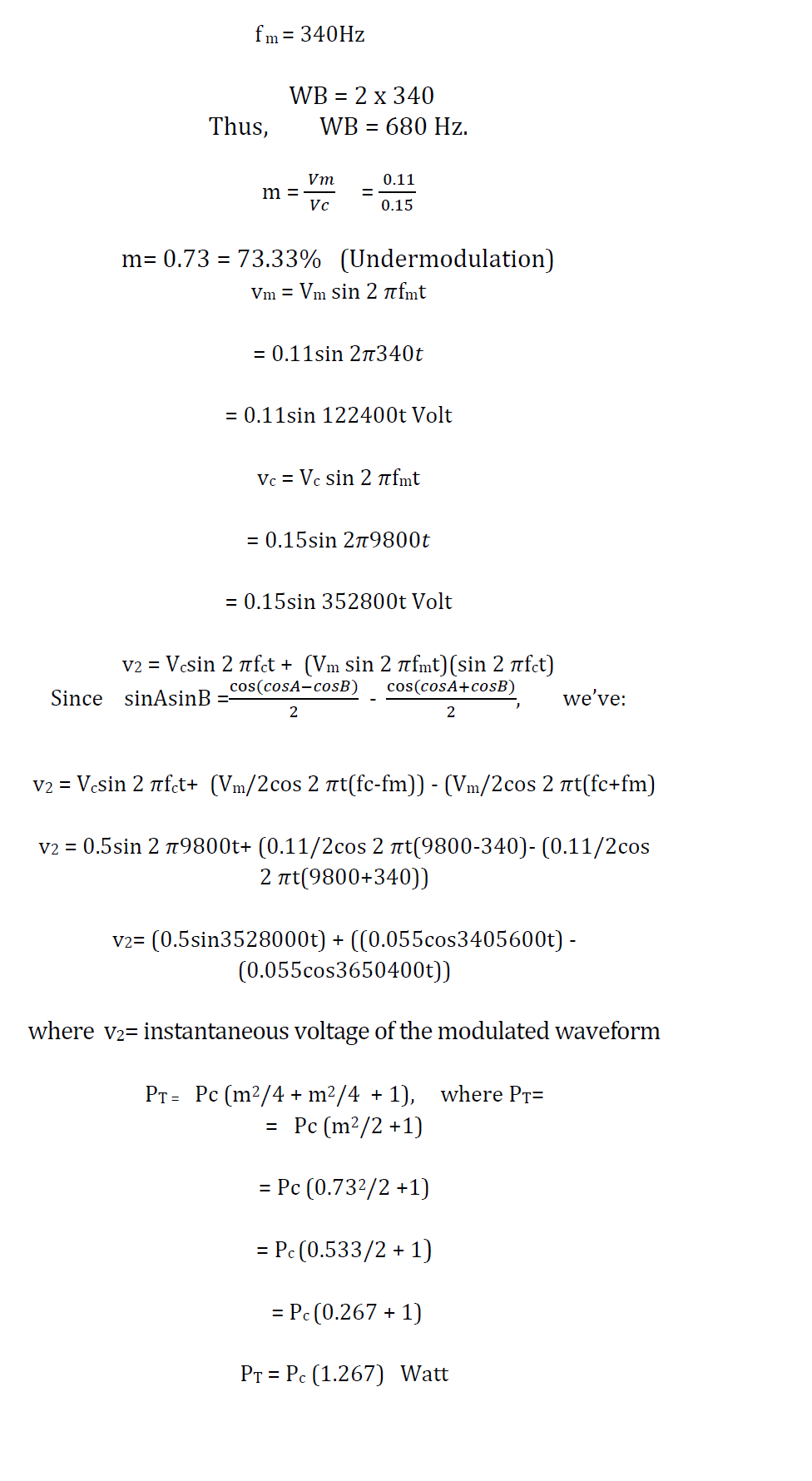
Transmission bandwidth WB = 2 f_m

Conclusion

My voice (with amplitude 0.11V and frequency 340Hz) modulated a carrier ( with amplitude 0.15V and frequency 9800Hz) to produce a modulated signal with the following parameters:

• Bandwidth of transmission is 680kHz

• Modulation index, m is 73.33%. This is under modulation. The ratio of modulating signal amplitude to carrier amplitude was carefully chosen to avoid distortion. Any value of m above 100%(called over modulation) causes distortion

The instantaneous value of my modulating signal at a given time is as given below:

v_m = 0.11sin 122400t Volt

The instantaneous value of my carrier signal at a given time is as given below:

v_c = 0.15sin 352800t Volt

The instantaneous voltage of the modulated waveform at a given timeis as given below: 

v₂= (0.5sin3528000t) + ((0.055cos3405600t) - (0.055cos3650400t))

Effective power distribution in the AM waveform is as given below: 

P_T = P_c (1.267) Watt

To demodulate the modulated signal in order to recover back a sine wave (i.e the frequency of my voice) in the MATLAB IDE

A modulated signal cannot be heard by human ear. This is because it is transmitted at the frequency of carrier signal and this is not audible by human ear. For the transmitted information to be heard by ordinary ear, it must be demodulated.

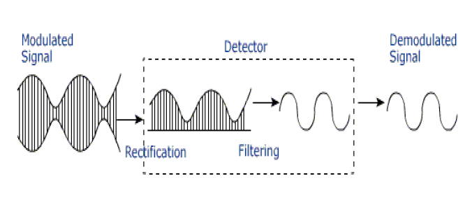
Thus, demodulation can be defined as a means of recovering information from modulated signal. 

There are basically two types of modulation: 

• Coherent

• Incoherent

Coherent Demodulation

This involves multiplying the AM signal by a sinusoid of exactly the same frequency and phase

Incoherent Demodulation

This does not involve multiplying the AM signal by a sinusoid

Importance of Demodulation

Demodulation is important because if it is not done, after filtering, the positive and negative envelopes will cancel each other so the original information cannot be recovered. This is because the modulation enveloped on the positive and negative sides are 180^o out of phase. (TutorVista.Com,n.d.).

Figure 14: Showing Demodulation Action (TutorVista.Com,n.d.)

Important Characteristics of a Demodulator

• Linearity

• Signal handling capacity

• Sensitivity

Linearity

This is the ability of a demodulator to produce an output with an amplitude of very insignificant variation to the amplitude of its input.

Signal handling capacity

This is a measure of signal amplitudes that a demodulator can accept without distortion.

Sensitivity

This is a measure of how much useful output is recovered when input is fed in. (TutorVista.Com,n.d.).

Demodulation in MATLAB IDE

Coherent Demodulation: which involves multiplying the modulated AM signal by a sinusoid of exactly the same frequency and phase of carrier signal was adopted in this work.

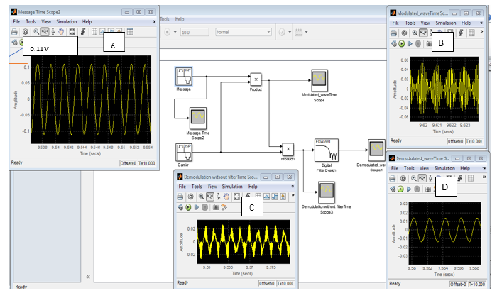
The procedure is as followed in modulation described above method but this time the same carrier frequency which was used for modulation was now multiplied with the modulated signal and the result was filtered (using digital low pass filter)as shown in Figure16 below.

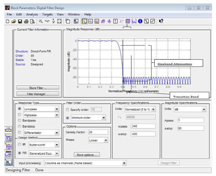
Figure 15: Showing Chosen Parameters of Low Pass Filter

Figure16: Setup Displaying Demodulation Building Blocks

The parameters of the digital low pass filter were chosen as seen in figure15 above and enumerated below:

• Uni Hz

• Frequency pass(F_pass) 0.340kHz(my voice fundamental frequency)

• Frequency stop(F_stop) 0.40kHz(frequency above my voice fundamental frequency)

• F = 1/T, i.e Sampling frequency Fs = 40000Hz

• Fs> 2(Fc + BW), where BW is the bandwidth of the original modulated signal       

• Generalized equiripple FIR was chosen as shown in Figure 15 above as my filter because it gave the maximum stopband attenuation. The higher the stopband attenuation the better the filtering ability of the filter

• Transition band for the filter was chosen to be very small (i.e. 0.4 – 0.34 = 0.06Hz) because the thinner it is the more nearly ideal the filter become

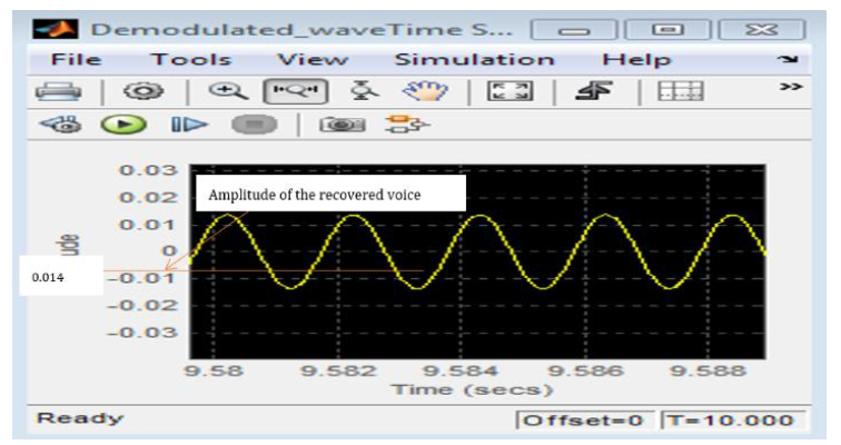
Figure 17: Demodulated Voice

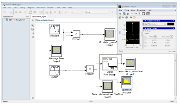
Figure 18: Showing Spectrum Analyser with The Display of the Frequency of Demodulated Signal

Figure 19: Clear Picture of Demodulated Signal Frequency from Spectrum Analyser

From Figure16 given above, it is shown through the Time Scope labelled ‘C’ that after the demodulation of modulated signal, some ripples were still present in the signal. The ripples were removed through the use of FIR filter. The final output is as shown in the Time Scope labelled ‘D’ in the same Figure16. And the signal is a replica of my voice but has suffered a lot of attenuation because its new amplitude has reduced to 0.014V.

1. Rose, Jay. “Range finder.” DPlay, 2008, http://www.dplay.com/tutorial/bands/. Accessed March 2014.

2. Adediran, Yinusa A. Applied electricity. 1st ed., Finom, 2000, pp. 192–193.

3. “Mixed-frequency signals.” All About Circuits, 2012, http://www.allaboutcircuits.com. Accessed March 2014.

4. “Graphs of sine, cosine and tangent.” Math Is Fun, 2011, http://www.mathsisfun.com/algebra/trig-sin-cos-tan-graphs.html. Accessed March 2014.

5. “Amplitude modulation fundamentals.” Data Communications, n.d., http://www.pa2old.nl/files/am _fundamentals.pdf. Accessed March 2014.