
+91 6002993949
submission@iarconsortium.org
Open Access
ISSN (Print) : 2788-9459
ISSN (Online) : 2788-9467
This study consists of a comprehensive analysis of thirteen soil samples taken from the Laylan region of Kirkuk City, Iraq, with respect to physical parameters such as texture, Atterberg limits, water content material, and dry density. We created maps using various interpolation techniques in a GIS program, which includes IDW, Kriging, and Spline. This enabled us to observe the variations in these characteristics across different geographical locations. We used the moisture density meter version HS-5001EZ to degree each the dry and moist densities. Nonlinear regression models outperformed linear ones in detecting stronger connections between physical characteristics, indicating the complexity of soil behaviour. The plastic limit, water content, and liquid limit exhibit weak positive correlations, emphasizing the complicated relationships between these soil parameters. The strong correlation between the amounts of sand and silt indicated the cohesive distribution of the soil samples, which is a significant finding. In addition, nonlinear regression approaches revealed a relatively strong correlation between dry density and water content This provided us with new insights into the impact of moisture on soil stability and compaction. Using GIS interpolation methods, this study investigates soil properties in the Laylan neighborhood of Kirkuk City. This study examines the organic matter composition, pH, and electrical conductivity. This study creates maps of distribution, identifies areas with high soil fertility, and displays these maps using geographic information systems
Accurate and strategic farming depends heavily on the physical and chemical characteristics of the soil. Regarding farming, soil texture is the primary physical characteristic of the soil [1]. Effective soil management requires close observation of the qualities of the soil [2], [3]. Soils consist of intricate combinations of minerals and organic compounds, interspersed with pore spaces saturated with water [4].
In this context, ground measurements have long been used to assess soil texture or water status, but they are expensive, time-consuming processes and insufficient due to the complexity of accurately monitoring spatiotemporal fluctuations in soil moisture. AS a consequence, scientific studies have put much work into creating remote sensing products, expecting to increase the precision and temporal and spatial coverage of these observations when evaluating water resource management and hydrological applications [5]–[9].Soil texture affects a variety of physical and chemical parameters, including permeability, adsorption and absorption characteristics, cation exchange, moisture-holding capacity, and soil fertility[10]. It is difficult and expensive to conduct soil property mapping in remote places using typical survey methods [11], [12].
However, the development of remote sensing (RS), modelling, and geographic information systems (GISs) has facilitated anticipating soil qualities across landscapes, even in previously unreachable areas [13], [14]. To forecast soil qualities across landscapes, there is a growing need to use technologies such as GIS, RS, and modelling approaches [11], [12], [15].
Regular soil surveys also gather data on the physical and chemical properties of the soil at the component level to create maps that show how these properties are distributed across different areas [16]. The mapping of soil properties can be difficult in locations with low agricultural potential where traditional soil survey procedures can be time-consuming and expensive, especially in isolated areas [15] . Estimating soil properties using remote sensing data has been the concern of numerous strategies in the last numerous a long time [17] . One useful tool for studying earth resources, especially soil quality, has been the development of remote sensing technology in the last 30 years [18]. The spatial and integrated images of many land attributes that RS are beneficial because they provide a more thorough understanding of the landscape as a whole [19].
For several academic disciplines, including hydrology, ecology, meteorology, irrigation effectiveness, crop pattern management, and soil categorization, soil texture data are considered essential [20] . Moreover, the commonplace techniques for estimating soil residences from RS facts include regression analysis models and geostatistical techniques [21], [22]. The extracted information may be organized, analysed, and stored in databases using geographic information systems (GIS) [14].
The soil parameters and distribution of the retrieved statistics had been modeled and mapped the use of GIS via interpolation techniques [12] . Numerous factors, consisting of soil heterogeneity, interpolation techniques, and sampling, might affect the best of a map produced using such geostatistical strategies [13]. These methods, which take into account the precise positions of the data points in the sample, are known as spatial interpolation techniques, and they differ from common statistical approaches [23]– [25]. Unfortunately, gathering and interpreting data on soil physical parameters with a high level of accuracy is difficult due to time constraints and the unpredictable variability of soil deposits. Thus, the main objective of this study is to identify the most reliable correlations between indicators of clay soil properties and characterize soil fertility with in the study area. These associations are characterized using the ordinary least squares method. By utilising interpolation methods grounded in Geographic Information System (GIS) approaches, this study aims to examine the importance and spatial distribution of crucial soil parameters in the Laylan area of Kirkuk City, Northern Iraq.
Study area
The study area is located in the city of Laylan, within the Kirkuk Governorate in north-central Iraq. The Laylan boundary spans from longitude of 44° 20’ to 44° 45’ and from latitude of 35° 09’ to 35° 25’. The area's terrain is mostly flat, with a few scattered hills stretching southwest towards the Jambur anticline at an elevation of 243–402 meters above the sea level [26]. The total land area of Laylan is approximately 691 Km2.Due to its significant oil production, it maintains considerable economic importance. It is situated approximately 274 Km from the capital Baghdad and approximately 19 Km from Kirkuk. The Kirkuk Cement factory is located within its limits. The Kirkuk structure borders the area to the northeast, and the Jambur anticline borders to the southwest [27]. The ephemeral streams Shireen and Mamsha form the southern and western boundaries, respectively, while Shireen forms the western and northwestern boundaries, respectively[28], [29].
Figure 1. Map of the study area (satellite imagery
The methodology of this study included field measurements and satellite data using GIS techniques (interpolation techniques) and a linear regression model to determine soil properties (physical and chemical) and percentages of sand, silt and clay.The texture of the soil, Atterberg limits, dry density, and water content are considered. The general methodology is illustrated in Figure (2).
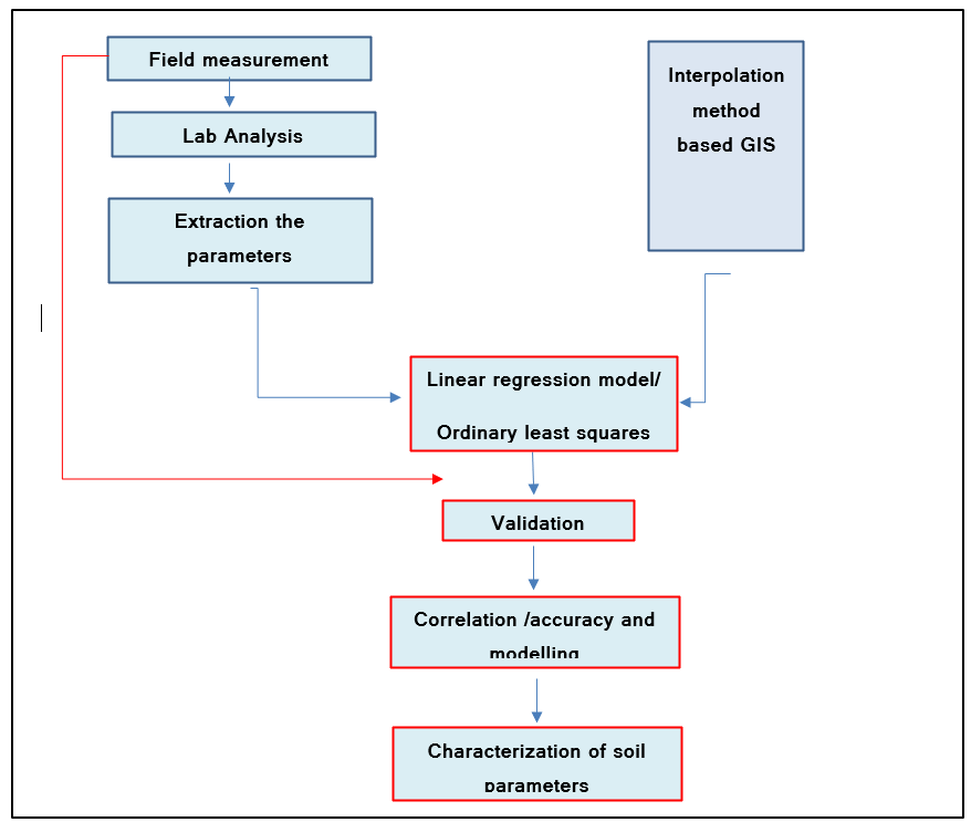
Figure 2. Flow chart of the applied method.
Field measurements and soil analysis.
Thirteen sites were extracted from the research location. These sites were located in the Laylan region, Kirkuk, Iraq. The coordinates were pinpointed by a portable GPS device (±3.6). An HS-5001EZ moisture-density meter was used to determine the dry density and the water content. On the other hand, the physical characteristics of the soil were extracted after drying the samples in a laboratory oven at 100°C for 24 hours prior to laboratory analysis. To calculate the Liquid Limit, the Casagrande three-point approach was used[19]. A soil thread 3 mm in diameter was used to determine the plastic limits (PLs)[30]. All measurements were completed in accordance with the standards of the American Society for Testing and Materials.
Table 1. measurements of Liquid Limit and Plastic Limit
NO. | Code | X | Y | Liquid Limit |
| Plastic Limit |
1 | 41 | 454175 | 3910651.9 | 28 |
| 15 |
2 | 1 | 453945 | 3908513.1 | 28 |
| 16.66 |
3 | 2 | 454661 | 3908556.7 | 29.5 |
| 16.7 |
4 | 3 | 454127 | 3909831.6 | 20 |
| 0 |
5 | 4 | 455414 | 3909571.7 | 24.05 |
| 0 |
6 | 5 | 455273 | 3910415.2 | 19.8 |
| 0 |
7 | 6 | 455066 | 3909919.2 | 25.3 |
| 0 |
8 | 7 | 454723 | 3909627.2 | 31.2 |
| 17.5 |
9 | 8 | 452315 | 3916189.7 | 26.8 |
| 0 |
10 | 9 | 453268 | 3916539.7 | 29.5 |
| 0 |
11 | 10 | 452038 | 3915780.1 | 22.2 |
| 16.8 |
12 | 11 | 450743 | 3914829.3 | 25.9 |
| 15 |
13 | 21 | 450231 | 3914826.4 | 27.2 |
| 15 |
Interpolation methods
Many fields struggle to generate continuous surfaces from non-normally distributed data. Many different approaches can do this, but picking the one that most closely mimics the real surface is tricky [31].
The set of point data properties determines the relative merits of various methods [31]. The process of spatial interpolation involves using measurements taken at nearby sites (known values of sampled points) to estimate the unknown attribute values at unmeasured or unsampled places [32]. Interpolation methods have been used in several fields involving the Earth's surface because they are critical tools for estimating spatially continuous data [32].
In this study, we applied three interpolation methods
Inverse distance weighted
Inverse distance weighted (IDW) is a method of precise local deterministic interpolation [33]. According to IDW, the value at a site that has not been sampled is just the average of all the sampled points within a certain neighborhood of that location, weighted by distance [34]. As a result, IDW assumes that points in close proximity to the forecast site have a greater impact on the anticipated value than points further away [32]. IDW uses:
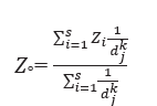
(1)
Where: Z0 denotes the expected value at a nonsampled site and Zi signifies the observed value, di represents the distance between the prediction location and the measurement location, S represents the number of sample points measured within the surrounding area, K is the power parameter determining how quickly the weights decrease as the distance increases.
Although IDW is a rapid lightning interpolation method, it is highly vulnerable to data clustering and outliers. Moreover, this method does not allow for an implicit assessment of forecast accuracy[32].
Kriging
Like IDW, kriging interpolation uses the measured values in an area to forecast a spot that has not yet been measured [35]. On the other hand, Kriging considers both the measured points' relative positions to the predicted location and their general spatial arrangement when determining weights [32].
According to Kriging, surface variation can be explained by observing the direction or distance between sample points, which are spatially correlated [34]. The spatial arrangement of the weights can only be utilized once the spatial autocorrelation of the empirical semivariograms has been assessed[32].
There are several possible models for semivariograms, including circular, spherical, exponential, Gaussian, and linear models[32]. For each point, kriging finds the output value by fitting a mathematical function to all points within a given radius or a set number of points. The data are best suited for kriging when there is a direction bias or a spatially linked distance[32]. The interpolation of Kriging method can be expressed as Eq.2:
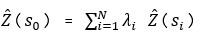
2
Where: Z(Si) represents the i-th position of the measured value, i represents the i-th position of the unknown weight, S0 represents the projected location, and N represents the number of measurements.
Table 2. measured data for density parameter
FID_ | density | RASTER VALU |
3 | 1.498 | 1.8403161 |
6 | 1.698 | 1.7449644 |
8 | 1.61 | 1.825711 |
11 | 1.614 | 1.586308 |
Spline
Another often employed local interpolation technique is bicubic splines, also referred to as splines[34]. Spline interpolation is a method that uses a mathematical function to estimate the elevation of a particular point. This function is designed to minimize the curvature of the surface, resulting in a smooth surface that precisely passes through the given input points[32]. Spline functions are natural extensions of polynomials due to their advantageous properties as approximation and interpolation functions[36].
Linear regression model
The statistical method of regression analysis estimates the value of a dependent variable by taking into account independent variables and establishing their relationship[22]. There are several types of regression models, such as linear, multilinear, and nonlinear regressions. The function of linear regression is given as Eq. 3 [37]:
(3)
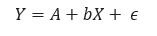
The dependent variable is denoted as Y, the independent variable as X, the intercept as A, the slope as B, and the error term as ϵ .
Soil field measurements were taken at 13 locations across the Laylan region in Kirkuk using an HS-5001EZ moisture density gauge. The following results have been determined:
Laboratory and statistical analysis
An analysis of the specific sizes of the thirteen soil samples revealed that the percentage of gravel was generally low, ranging from 0 to 8% in most cases. However, three of the sites had gravel percentages of 21.3%, 34.7%, and 38.1%, respectively. The sand content varied from 2.32% to 25.86% in most samples, except for two locations where it was notably higher at 55.24% and 50.02%, respectively. Silt was identified as the predominant component in the majority of areas.
Atterberg Limits
The boundary delineating different physical states of sediments was established using the Atterberg limits. Analysis of the Atterberg limits revealed that the liquid limit ranged from 19.8% to 31.2%, with an average of 25.95%. The plastic limit values varied from 0% to 17.5%, with an average of 8.66%. The plasticity index, representing the difference between the liquid limit and plastic limit, ranged from 5.4% to 29.5%. Most soil samples exhibited a notable presence of silt, resulting in plasticity index values ranging from low to moderate. The following table illustrate the plasticity index of soil.
Table 3 Range of Plasticity index
PI Value | Description of Plasticity |
0 | Non Plastic |
< 7 | Less Plastic |
7 – 17 | Medium Plastic |
7 > | High Plastic |
Partial analysis of the soil using interpolation techniques
The interpolation technique was utilized to partition the physical properties into five distinct zones to analyse their spatial arrangement. These zones range from very low to very high. White hues represent areas with a higher concentration, whereas green hues indicate areas with a lower proportion. Fig.3 shows the distribution of clay and gravel the distribution of clay ranging from 0% to 14.48% using three methods of interpolation and identifies the distribution of gravel percentages ranging from 0% to 38.1%.
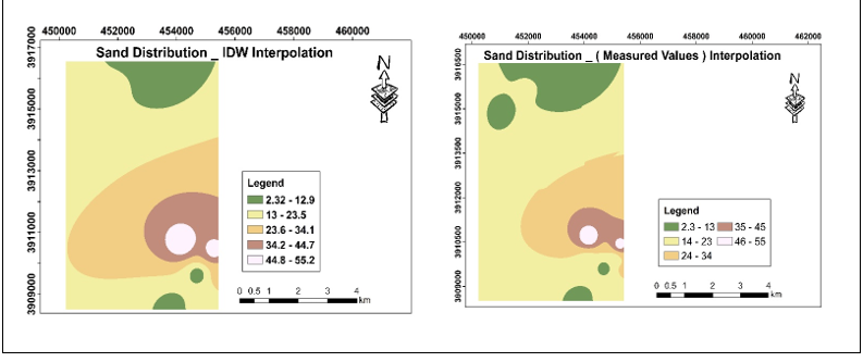
Fig.4 shows the representation of sand and silt the distribution of sand ranging from 2.32% to 55.24% and distribution of silt content ranging from 6.7% to 96.08%. Fig.5 shows the distribution of moisture and density measurement, the representation of moisture measurements taken from the field using HS-5001EZ moisture density gauge, which showed that the moisture content ranged from 2 to 8.2% and distribution of dry density measurements that was taken by the same device, which showed that the dry density ranged from 1.49 to 1.992 g/m3. Fig.6 shows the distribution of Liquid Limit and Plastic Limit, the distribution of LL ranging from 19.8 to 31.2 and distribution of the PL ranging from 0 to 17.5.
The liquid limit (LL) is the moisture percentage at which the soil transitions from a liquid to a plastic state. Similarly, the plastic limit (PL) represents the moisture levels, expressed as a percentage, at which the soil transitions from a plastic to a semisolid state.
In the clay parameter, the best method is IDW, where the value of R2 is 0.62. In the gravel parameter, the same method gives the best result, where the value of R2 is 0.38. In terms of sand and silt parameters, the IDW method also produces the best results, with R2 values of 0.71 and 0.52, respectively. In the water content parameter, the IDW method is the best, with a value of R2 of 0.27, whereas in dry density, the Kriging method is the best, with a value of R2 of 0.19. For the liquid limit and plastic limit parameters, the spline method is the best for the liquid limit, where the value of R2 is 0.94, while in the plastic limit, the IDW method gives the best result, where the value of R2 is 0.25.
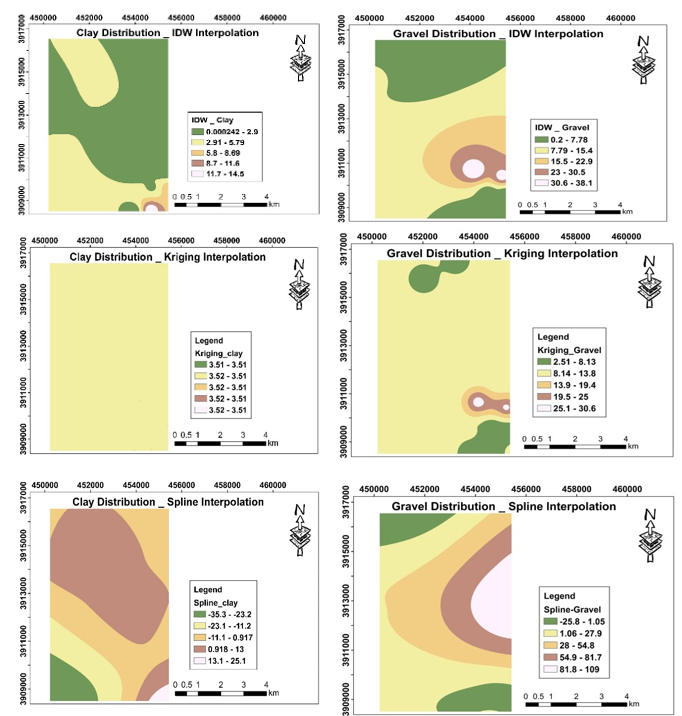
Figure 3. Representation of Clay & Gravel
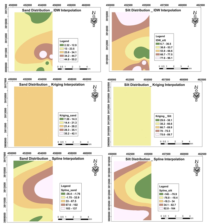
Figure 4. Representation of Sand & Silt
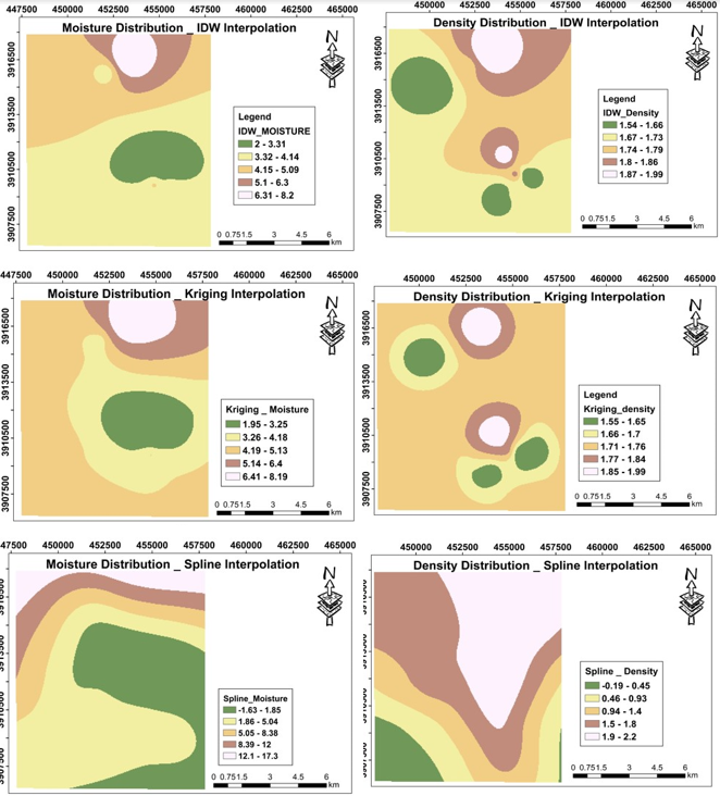
Figure 5. Representation of Moisture & Density
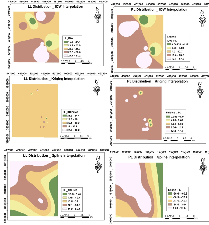
Figure 6. Representation of LL & PL
Validation and model generation
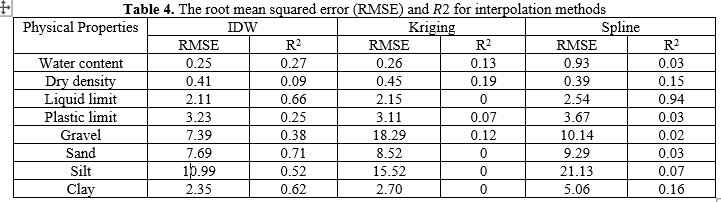
After producing maps of physical properties and percentages of soil texture using the interpolation methods, to ensure the accuracy of the results, 30% of the soil samples (testing data) were used to determine the difference between a field value and a value calculated by the interpolation methods. Table 4 shows the RMSEs of the physical properties obtained via interpolation methods.
The validation shows that generally, the IDW method is the best one where the value of R2 is higher than the other two methods except in dry density and liquid limit, where the Kriging and Spline methods, respectively, are giving better results than the IDW method.
The following maps show the difference between measured and calculated values
A linear and nonlinear regression model was used to correlate and characterize the physical properties of the soil. Tables 5 & 6 show the relationships between soil properties such as soil texture (gravel, sand, silt, and clay), water content, dry density and Atterberg limits (LL, PL & PI). As shown in Table 5, while most of the parameters were unrelated to any of the other parameters, the correlation results revealed a significant positive correlation with the plasticity index and silt content (0.817 and 0.952, respectively). As shown in Table 6, the correlation results revealed a significant positive correlation with dry density, plasticity index, sand and silt (0.663, 0.82, 0.736 and 0.952, respectively). Nonlinear results are regularly higher than linear results for numerous reasons, particularly in the context of modeling and reading complex systems Interactions, Accuracy and Flexibility.
Based on these statistical relationships, we can say that linear relationships don't usually show a positive correlation. The three-parameter correlation (the platic limit, gravel, and sand) is the only one that does. The plastic limit and the plasticity index do, however, show a positive correlation. When the plastic limit increases, it will have an effect on the plasticity index, whereas in non-linear relationships, we find the best results for parameters compared to linear relationships.For example, there was a correlation between water content and dry density, as well as a significantly positive correlation between plastic limit and plasticity index, gravel and sand, gravel and silt, and sand and silt. The rate of increase or decrease can change as one variable changes.
Table 5. Linear relationship between the physical properties of the soil
Physical properties | Water content | Dry density | L.L | P.L | P.I | gravel | sand | silt | clay |
Water content | 1 |
|
|
|
|
|
|
|
|
Dry density | 0.01 | 1 |
|
|
|
|
|
|
|
L.L | 0.11 | 0.14 | 1 |
|
|
|
|
|
|
P.L | 0.04 | 0 | 0.22 | 1 |
|
|
|
|
|
P.I | 0.15 | 0.01 | 0 | 0.82 | 1 |
|
|
|
|
Gravel | 0 | 0.35 | 0.02 | 0.03 | 0.02 | 1 |
|
|
|
Sand | 0.05 | 0.21 | 0 | 0.03 | 0.03 | 0.74 | 1 |
|
|
Silt | 0.17 | 0.12 | 0.08 | 0 | 0 | 0.86 | 0.95 | 1 |
|
Clay | 0 | 0.06 | 0.01 | 0.01 | 0 | 0.12 | 0.01 | 0 | 1 |
Using SPSS (Statistical Package for the Social Sciences) software, we calculate non-linear relationships by inserting dependent and independent variables and producing an R2 value. We have different methods for calculating the R2 value in non-linear relationships, including quadratic, compound, growth, logarithmic, cubic, s, exponential, inverse, power, and logistic. We select the best method based on the value of R2, where a higher value is acceptable.
Table 6. Nonlinear relationships between the physical properties of the soil
Physical properties | Water content | Dry density | L.L | P.L | P.I | gravel | sand | silt | clay |
Water content | 1 |
|
|
|
|
|
|
|
|
Dry density | 0.66 | 1 |
|
|
|
|
|
|
|
L.L | 0.15 | 0.14 | 1 |
|
|
|
|
|
|
P.L | 0.11 | 0.09 | 0.22 | 1 |
|
|
|
|
|
P.I | 0.25 | 0.14 | 0 | 0.82 | 1 |
|
|
|
|
Gravel % | 0.22 | 0.06 | 0.17 | 0.02 | 0 | 1 |
|
|
|
Sand % | 0.46 | 0.06 | 0.12 | 0.01 | 0 | 0.74 | 1 |
|
|
Silt % | 0.39 | 0.05 | 0.16 | 0.02 | 0 | 0.86 | 0.96 | 1 |
|
Clay % | 0.01 | 0.09 | 0 | 0 | 0 | 0.12 | 0.01 | 0 | 1 |
The investigation of soil physical parameters, including texture, Atterberg limits, water content, and dry density, was conducted rigorously through the collection and analysis of 13 soil samples. These samples were subjected to mapping using various interpolation methods, such as IDW, kriging, and spline methods. The dry density and moisture were measured using an HS-5001EZ moisture density meter, revealing a range of dry densities from 1.49 to 1.992 g/m³ and moisture levels spanning from 2% to 8.2%. Notably, the majority of the samples exhibited a substantial silt content, contributing significantly to the plasticity index falling within the low to medium plasticity range.
Further analysis revealed compelling correlations within the data. The liquid limit, plastic limit, and specific gravity displayed weak positive correlations with the water content, indicating subtle but observable relationships between these parameters. Moreover, the gravel content exhibited fantastic fine correlations with each the sand and silt concentrations, as evidenced by R values of 0.736 and 0.859, respectively. These findings underscore the interplay among different soil components and their effect on each other's concentrations.
Comparative analysis among linear and nonlinear regression models discovered that the latter yielded stronger correlations among physical parameters. This suggests the complexity of soil behavior and the efficacy of nonlinear modelling in capturing these details more accurately. Additionally, the LL and PL demonstrated weak positive correlations with the water content, further highlighting the subtle relationships among the soil properties.
One of the significant findings was the robust relationship located among sand and silt concentrations, indicating a cohesive nature of their distribution inside the soil samples. Moreover, the link between dry density and moisture showed a rather strong correlation when analyzed using nonlinear regression techniques, with a R value of 0.663. This finding provides valuable insights into the vital moisture-density relationship, which is essential for comprehending soil compaction and stability.
In essence, this study very well explored soil characteristics, interpreting complicated relationships and providing precious insights into soil behavior. These findings have the capability to inform numerous fields, including agriculture, geology, and environmental science.
U. Barman, R. D. Choudhury, N. Talukdar, P. Deka, I. Kalita, and N. Rahman, “Predication of soil pH using HSI colour image processing and regression over Guwahati, Assam, India,” J. Appl. Nat. Sci., vol. 10, no. 2, pp. 805–809, 2018. DOI:10.31018/jans.v10i2.1701
A. Erturk, U. Alganci, A. Tanik, and D. Z. Seker, “Determination of land-use dynamics in a lagoon watershed by remotely sensed data.,” 2012. https://research.itu.edu.tr/en/publications/determination-of-land-use-dynamics-in-a-lagoon-watershed-by-remot
A. Okatan, M. Aydin, A. Usta, and M. Yilmaz, “Effects of land use type on hydro-physical properties of soils in the Torul dam basin-Gumushane, Turkey,” Fresenius Environ. Bull., vol. 19, no. 12b, pp. 3230–3241, 2010.
A. H. Taqi, Q. A. M. Al Nuaimy, and G. A. Karem, “Study of the properties of soil in Kirkuk, IRAQ,” J. Radiat. Res. Appl. Sci., vol. 9, no. 3, pp. 259–265, 2016. https://www.researchgate.net/publication/286291115_Effects_of_land_use_type_on_hydro-physical_properties_of_soils_in_the_torul_dam_basin-gumushane_Turkey
M. Zribi et al., “CAROLS: A new airborne L-band radiometer for ocean surface and land observations,” Sensors, vol. 11, no. 1, pp. 719–742, 2011. doi: 10.3390/s110100719.
W. Korres et al., “Spatio-temporal soil moisture patterns–A meta-analysis using plot to catchment scale data,” J. Hydrol., vol. 520, pp. 326–341, 2015. DOI: 10.1016/j.jhydrol.2014.11.042
T. K. Alexandridis et al., “Spatial and temporal distribution of soil moisture at the catchment scale using remotely-sensed energy fluxes,” Water, vol. 8, no. 1, p. 32, 2016.
L. Brocca, F. Melone, T. Moramarco, and R. Morbidelli, “Spatial‐temporal variability of soil moisture and its estimation across scales,” Water Resour. Res., vol. 46, no. 2, 2010. https://agupubs.onlinelibrary.wiley.com/doi/epdf/10.1029/2009WR008016
N. N. Baghdadi, M. El Hajj, M. Zribi, and I. Fayad, “Coupling SAR C-band and optical data for soil moisture and leaf area index retrieval over irrigated grasslands,” IEEE J. Sel. Top. Appl. Earth Obs. Remote Sens., vol. 9, no. 3, pp. 1229–1243, 2015. DOI:10.1109/IGARSS.2016.7729919
S. Makabe, K.-I. Kakuda, Y. Sasaki, T. Ando, H. Fujii, and H. Ando, “Relationship between mineral composition or soil texture and available silicon in alluvial paddy soils on the Shounai Plain, Japan,” Soil Sci. plant Nutr., vol. 55, no. 2, pp. 300–308, 2009. DOI:10.1111/j.1747-0765.2008.00352.
A. B. McBratney, M. L. M. Santos, and B. Minasny, “On digital soil mapping,” Geoderma, vol. 117, no. 1–2, pp. 3–52, 2003. https://doi.org/10.1016/S0016-7061(03)00223-4
C. E. Akumu et al., “GIS-fuzzy logic based approach in modeling soil texture: Using parts of the Clay Belt and Hornepayne region in Ontario Canada as a case study,” Geoderma, vol. 239, pp. 13–24, 2015. https://doi.org/10.1016/j.geoderma.2016.07.028
M. A. Shareef, M. H. Ameen, and Q. M. Ajaj, “Change detection and GIS-based fuzzy AHP to evaluate the degradation and reclamation land of Tikrit City, Iraq,” Geod. Cartogr., vol. 46, no. 4, pp. 194–203, 2020. DOI:10.3846/gac.2020.11616
H. G. Maarez, H. S. Jaber, and M. A. Shareef, “Utilization of Geographic Information System for hydrological analyses: A case study of Karbala province, Iraq,” Iraqi J. Sci., pp. 4118–4130, 2022. DOI:10.24996/ijs.2022.63.9.39
M. A. Shareef, N. D. Hassan, S. F. Hasan, and A. Khenchaf, “Integration of Sentinel-1A and Sentinel-2B Data for Land Use and Land Cover Mapping of the Kirkuk Governorate, Iraq.,” Int. J. Geoinformatics, vol. 16, no. 3, 2020. https://journals.sfu.ca/ijg/index.php/journal/article/view/1783
A.-X. Zhu, F. Qi, A. Moore, and J. E. Burt, “Prediction of soil properties using fuzzy membership values,” Geoderma, vol. 158, no. 3–4, pp. 199–206, 2010. https://doi.org/10.1016/j.geoderma.2010.05.001
E. S. Mohamed, A. Ali, M. El-Shirbeny, K. Abutaleb, and S. M. Shaddad, “Mapping soil moisture and their correlation with crop pattern using remotely sensed data in arid region,” Egypt. J. Remote Sens. Sp. Sci., vol. 23, no. 3, pp. 347–353, 2020. DOI:10.1016/j.ejrs.2019.04.003
S. Periasamy, D. Senthil, and R. S. Shanmugam, “A soil texture categorization mapping from empirical and semi-empirical modelling of target parameters of synthetic aperture radar,” Geocarto Int., vol. 36, no. 5, pp. 581–598, 2021, doi: 10.1080/10106049.2019.1618924. DOI:10.1080/10106049.2019.1618924
V. F. Salahalden, M. A. Shareef, and Q. A. A. Nuaimy, “Red Clay Soil Physical and Chemical Properties Distribution Using Remote Sensing and GIS Techniques in Kirkuk City, Iraq,” Iraqi Geol. J., vol. 57, no. 1, pp. 194–220, 2024, doi: 10.46717/igj.57.1A.16ms-2024-1-27. DOI:10.46717/igj.57.1a.16ms-2024-1-27
M. T. Esetlili and Y. Kurucu, “Determination of Main Soil Properties Using Synthetic Aperture Radar,” Fresenius Environ. Bull., vol. 25, no. 1, pp. 23–36, 2016. https://www.researchgate.net/publication/299448469_DETERMINATION_OF_MAIN_SOIL_PROPERTIES_USING_SYNTHETIC_APERTURE_RADAR
S. Sridevy et al., “Mapping of Soil Properties Using Machine Learning Techniques,” Int. J. Environ. Clim. Chang., vol. 13, no. 8, pp. 684–700, 2023. DOI:10.9734/ijecc/2023/v13i81997
C. da Silva Chagas, W. de Carvalho Junior, S. B. Bhering, and B. Calderano Filho, “Spatial prediction of soil surface texture in a semiarid region using random forest and multiple linear regressions,” Catena, vol. 139, pp. 232–240, 2016. https://doi.org/10.1016/j.catena.2016.01.001
A. M. Raheem, N. Q. Omar, I. J. Naser, and M. O. Ibrahim, “GIS implementation and statistical analysis for significant characteristics of Kirkuk soil,” J. Mech. Behav. Mater., vol. 31, no. 1, pp. 691–700, 2022. DOI:10.1515/jmbm-2022-0073
A. M. Raheem, I. J. Naser, M. O. Ibrahim, and N. Q. Omar, “Inverse distance weighted (IDW) and kriging approaches integrated with linear single and multi-regression models to assess particular physico-consolidation soil properties for Kirkuk city,” Model. Earth Syst. Environ., pp. 1–23, 2023. DOI:10.1051/e3sconf/202342701005
A. M. Raheem and N. Q. Omar, “Investigation of distinctive physico-chemical soil correlations for Kirkuk city using spatial analysis technique incorporated with statistical modeling,” Int. J. Geo-Engineering, vol. 12, pp. 1–21, 2021. DOI:10.1186/s40703-021-00147-2
N. K. N. Abo-Khomra, O. S. I. Al-Tamimi, and A. A. Othman, “DRASTIC for Groundwater Vulnerability Assessment using GIS: A Case Study in Laylan Sub-Basin, Kirkuk, Iraq,” Iraqi Geol. J., vol. 55, no. 1, pp. 71–81, 2022, doi: 10.46717/igj.55.1B.7Ms-2022-02-23. DOI:10.46717/igj.55.1b.7ms-2022-02-23
Amin Beiranvand Pour, “Delineate the hydrological boundaries situation using the morphometric analysis and geological features: A case study of Laylan sub-basin, Kirkuk / NE Iraq,” IOP Conf. Ser. Earth Environ. Sci., vol. 1120, no. 1, 2022, doi: 10.1088/1755-1315/1120/1/012013.
A. A. Rasheed, “Evaluation of Groundwater in Laylan Basin, South East, Kirkuk,” Unpubl. Ph. D Thesis, vol. 205, 2019.
N. K. N. Abo-Khomra, O. S. I. Al-Tamimi, and A. A. Othman, “DRASTIC for groundwater vulnerability assessment using GIS: A case study in Laylan Sub-Basin, Kirkuk, Iraq,” Iraqi Geol. J., pp. 71–81, 2022. DOI:10.46717/igj.55.1b.7ms-2022-02-23
Z. Zolfaghari, M. R. Mosaddeghi, and S. Ayoubi, “ANN‐based pedotransfer and soil spatial prediction functions for predicting Atterberg consistency limits and indices from easily available properties at the watershed scale in western Iran,” Soil Use Manag., vol. 31, no. 1, pp. 142–154, 2015. https://doi.org/10.1111/sum.12167
C. Caruso and F. Quarta, “Interpolation methods comparison,” Comput. Math. with Appl., vol. 35, no. 12, pp. 109–126, 1998. https://doi.org/10.1016/S0898-1221(98)00101-1
Q. Tan and X. Xu, “Comparative analysis of spatial interpolation methods: An experimental study,” Sensors and Transducers, vol. 165, no. 2, pp. 155–163, 2014 https://www.researchgate.net/publication/279902313_Comparative_Analysis_of_Spatial_Interpolation_Methods_an_Experimental_Study.
D. F. Watson, “A refinement of inverse distance weighted interpolation,” Geo-processing, vol. 2, pp. 315–327, 1985. https://www.semanticscholar.org/paper/A-refinement-of-inverse-distance-weighted-Watson/05460f45dedb446b391889138aef84074986aead
P. A. Longley, M. F. Goodchild, D. J. Maguire, and D. W. Rhind, Geographic information science and systems. John Wiley & Sons, 2015. https://books.google.co.in/books/about/Geographic_Information_Science_and_Syste.html?id=C_EwBgAAQBAJ&redir_esc=y
M. A. Oliver and R. Webster, “Kriging: a method of interpolation for geographical information systems,” Int. J. Geogr. Inf. Syst., vol. 4, no. 3, pp. 313–332, 1990. https://doi.org/10.1080/02693799008941549
W. Freeden and W. Törnig, “On spherical spline interpolation and approximation,” Math. Methods Appl. Sci., vol. 3, no. 1, pp. 551–575, 1981, doi: 10.1002/mma.1670030139. https://doi.org/10.1002/mma.1670030139
M. A. Shareef, A. Toumi, and A. Khenchaf, “Estimation of water quality parameters using the regression model with fuzzy k-means clustering,” Int. J. Adv. Comput. Sci. Appl., vol. 5, no. 6, 2014. DOI:10.14569/IJACSA.2014.050624